RISC-V Vector Reduction Operations

When you need to reduce a vector into a scalar

Vector Instruction Sets implement multiple operation patterns. The most straightforward, basis of the Single Instruction Multiple Data (SIMD) paradigm, is the element wise pattern: the same operation (e.g. addition) is applied independently to each pair of corresponding elements from two input vectors (this pattern extends to any number of input vectors). When implemented in hardware, the vector datapath can be split into independent “lanes” which operate on independent sets of input elements and produce independent result elements. The lanes do not need to exchange data. This independence makes scaling the number of lanes more transparent since physical locality is not a prerequisite (at least for those operations).

The element wise pattern is illustrated by the figure below, using the naming convention adopted by RISC-V Vector: vector length, active body elements, masked elements, and tail¹ (The prestart section is not represented).

The element-wise pattern is complemented by another interesting pattern: the reduction (sometimes called horizontal operation). In the reduction pattern, multiple elements from the same vector input are combined together to produce a single result. The operation is performed between the elements of a vector rather than element-wise between two or more vectors.

Note: There exist other patterns, for example RVV 1.0 viota instruction (spec) or vcompress (spec) where multiple results are produced with an inter lane dependency (although this could be debated in the case of viota since the dependency is actually on the mask input).

In this post we will present RVV reduction scheme, the existing RVV 1.0 reduction operations, show a couple of examples and benchmarks them on RISC-V hardware (CanMV-K230).

Overview of Reduction Operation in RISC-V Vector

The basic pattern for an RVV reduction operation is:

v<redop>.vs vd, vs2, v1[, vm]

(RVV 1.0 specification) and it is illustrated by the figure below:

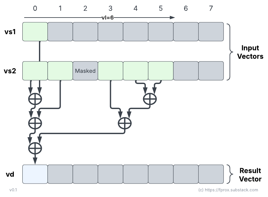
In RVV, the reduction pattern reduces a vector of input elements, vector register group vs2 (EMUL=LMUL), with a scalar input element read from the first element in vector register vs1 (EMUL=1). The RVV reduction pattern produces a single element result stored in the first element of vector register vd: vd[0] (EMUL=1). The other elements in vd are considered as part of the tail and follow the current tail policy. The operation can be optionally masked; the mask is used to select which elements of the vector register group vs2 take part in the reduction. Similarly the vector length, vl, determines the length of the body section (active elements) in vs2. The mask has no effect on the scalar source element read from vs1: vs1[0] is always part of the regression, even if all the elements in vs2 are masked off.

A zero vector length transforms the reduction operation into a no-operation:

“If vl=0, no operation is performed and the destination register is not updated.” (direct citation from RVV 1.0 specification)

Note: vs1 and vd are always considered as single vector register and not as possibly wider vector register group, i.e. they exhibit EMUL=1, regardless of the LMUL value. In particular this means that their register indices do not need to be aligned with the LMUL value; e.g. v3 is a valid vs1 source for a reduction even when LMUL >= 2.

Note: vd can overlap with either vs1, vs2 . It can even overlap the mask register when the operation is masked. This does not contradict RVV generic overlap constraints (spec) but rather derives from the fact that EMUL=1 for vd and that vd’s EEW is always at least as wide as any source EEW in any reduction operation.

Types of reduction operation in RVV

Now that we have viewed the high-level pattern of RISC-V Vector Reduction instructions, let’s review which operations are defined in RVV 1.0 to reduce a vector.

Integer reduction operations

RVV provides the following integer reduction operations:

• Logical Or, Xor, And: vred(or/xor/and).vs

• Single-width integer sum: vredsum.vs

• Widening integer sum: vwredsum[u].vs

• Integer minimum and maximum: vred(min/max)[u].vs

Widening integer reduction sum, vwredsum[u].vs, and min/max, vred(min/max)[u].vs, exist in both signed and unsigned variants (the mnemonics of the unsigned version use the suffix u).

For the widening sums, both the scalar element read from vs1 and the scalar result stored in vd are 2*SEW-bit wide. The elements read from vs2 are SEW-bit wide (EEW=SEW) and get zero extended (vwredsumu.vs) or sign extended (vwredsum.vs). Both integer reduction sums wrap on overflow.

Note/Reminder: EEW is the Effective Element Width, the actual width of elements. It can vary between operands, and between operands and destination. Its value is often derived from SEW (Selected Element Width, setting encoded in the field vsew of the vtype CSR and set through vset* instructions).

For all the reduction operations listed above the order of evaluation does not matter as the elementary 2-operand operations are associative and commutative: all orders return the same result.

Floating-Point reduction operations

RVV 1.0 also provides the following floating-point reduction operations:

• Floating-point minimum and maximum: vfred(min/max).vs

• Unordered Floating-point reduction sum: vf[w]redusum.vs

• Ordered Floating-point reduction sum: vf[w]redosum.vs

Floating-point reduction sum operations exist in 4 variants: ordered/unordered crossed with single-width/widening.

The floating-point formats supported by the reduction operation depend on which vector extension is actually enabled:

• double-precision is supported if Zve64d is present (and by extension if v is present)

• single-width single-precision is supported if Zve32f is present (which extends to Zve64f, Zve64d, and v). Widening reduction sums for single-precision are only supported if Zve64d is present (and by extension v).

• half-precision reductions are supported if Zvfh is present (since Zvfh depends on Zve32f, widening FP reduction sums from half to single precision are always supported if Zvfh is present since Zve32f is supported as well)

Note: As of April 2025, the (unratified) Zvfbfa Instruction Set Extension proposal version 0.1 (draft spec) excludes vector FP reduction operations. So no support for BFloat16 reduction operations is intended in RVV so far.

Floating-Point minimum / maximum reductions

The floating-point minimum (vfredmin.vs) and maximum (vfredmax.vs) reduction operations behave as their respective element-wise counterparts (vfmin.v* and vfmax.v*) which in turn behave as the scalar instructions fmin.* and fmax.* . They implement the minimumNumber (resp. maximumNumber) operation defined in the IEEE-754 standard for floating-point arithmetic: a number is selected over a NaN during the reduction, even a signaling NaN. Using this associative elementary operation in the reduction ensures that whatever the order of evaluation of the minimum (resp. maximum) the result is always the same.

Note: in its 2008 revision, the IEEE-754 standard defined non associative minNum and maxNum which would return a quiet NaN if either operand of an operation with a signaling NaN (see this report on why this was changed).

Floating-Point reduction sums

What is the difference between the ordered reduction vf[w]redosum.vs and the unordered version vf[w]redusum.vs ?

Note: for both widening variants vfwredosum.vs (ordered) and vfwredusum.vs (unordered) the elements from vs2 are read assuming EEW=SEW and are widened to 2*SEW prior to taking part into the actual reduction operation. The scalar input element vs1[0] and the result element in vd[0] both have EEW=2*SEW.

Floating-point addition is non-associative: (a + b) + c and a + (b + c) might return different results when evaluated with 2-operand floating-point addition with rounding. This property (quirk?) of Floating-Point addition, makes that there is no such thing as a single unique result for a sum of n floating-point values if a specific orderer is not attached.

Floating-Point ordered reduction sums

The ordered reduction sums, vf[w]redosum.vs, mandate a strict order of operation: the first element from vs2 must be added to the scalar element from vs1, and the rounded result is added to the second element from vs2, then rounded and added to the third elements …

This scheme exposes a linear order of reduction. It is not possible to parallelize the evaluation of an ordered FP reduction sum operation: it requires vl linearly dependent operations (some might be skipped if the element is masked off).

“The ordered reduction supports compiler autovectorization,” (direct citation from a Note in the RVV 1.0 standard)

Note: if there are no active element (e.g. vs2 is fully masked off), and vl > 0, vs1[0] gets copied to vd without change (no canonicalization of signaling NaN) and without raising any exception flags.

Floating-Point unordered reduction sums

The unordered FP reduction sum operations, vf[w]redusum.vs, offer more room for optimization. RVV 1.0 mandates that the unordered reduction needs to be implemented with a binary reduction tree. The precision on the intermediary nodes of the reduction tree is implementation defined and must be at least as wide as a SEW-bit format. Every rounding must be performed using the “currently active dynamic floating-point rounding mode” (a.k.a. the value set in the frm register). The root node is converted to the destination format (SEW-bit wide), so there could be double rounding for the final conversion in the case the root node is initially evaluated in a wider format. There is no ordering, nor shape constraint on the structure of the reduction tree: the implementation can be performed in any order.

We illustrated a valid example of unordered reduction scheme in the Figure below:

The space of possible implementations is very large. This is often disconcerting for a few different categories of people including hardware verification engineers and model developers (spike, QEMU, SAIL). How can you ensure an implementation is conformant if there is more than one valid answer ?

RVV 1.0 puts some constraint on the solution space: for a given (vl, vtype) pair, the structure of the reduction tree must be deterministic. This implies that an implementation cannot return different results on the same dataset and same configuration. The fact that the underlying structure must match a tree with binary operator nodes implementing 2-operand addition and rounding also means that it is possible to emulate the tree with scalar operations (although they might not correspond 1-to-1 to RISC-V instructions as they might be single width or widening even beyond the formats supported by any instructions).

The benefit of a wide solution space is that implementations can try to minimize the latency of the reduction by exploiting its intrinsic parallelism: it is legal to build a balanced binary tree with minimal depth, maximizing throughput and minimizing latency. But it is not mandated, so implementations choosing efficiency over speed can fallback on the same implementation for both ordered and unordered reductions (as the ordered reduction scheme is a valid scheme to implement unordered FP reduction sums).

In the illustrative examples we have shown previously, we get a 4-level deep unordered reduction versus an 8-level deep comb shape tree for the ordered version. Because of the non-associativity of the floating-point addition, these two schemes may not return the same result.

Two example use cases of RVV Reductions

We are now going to show some basic examples of the use of RVV reduction operations. The source code for those examples is available on github: rvv-examples:src/reduction.

Minimum of an array using RVV reductions

Let’s start by an example determining the minimum of an array of 32-bit signed integers:

// int32_t rvv_min(int32_t* inputVector, size_t len);
// a0: inputVector (memory address)
// a1: len (size, in number of elements)
rvv_min:
    // materializing INT32_MAX in a5
    li	a5,-2147483648
    addiw a5,a5,-1

    // loading INT32_MAX in the temporary minimum v16[0]
    vsetivli x0, 1, e32, m1
    vmv.v.x v16, a5

rvv_min_loop:
    // compute VL from AVL(a1) and store the result in a4
    vsetvli a4, a1, e32, m8
    // load VL new elements
    vle32.v v8, (a0)
    // perform reduction on v8 elements and v16[0]
    vredmin.vs v16, v8, v16
    // update AVL := AVL - VL 
    sub a1, a1, a4
    // update the array point inputVector += VL
    // since this is a byte address, the increment
    // is (VL << 2) = VL * 4
    sh2add a4, a4, a0
    // check whether AVL has reached zero or not, loop back if not
    bnez a1, rvv_min_loop

    // move the result from vector register to scalar register
    vmv.x.s a0, v16
    // sign extend to comply with RV64 ABI
    sext.w a0, a0
    ret

We use the usual loop strip-mining technique: at each loop iteration the program evaluates the vector length vl from the remaining application vector length (AVL). vl is given by whose results depends on AVL and the (micro-)architecture capabilities, including the implementation VLEN. The program loads vl new elements from the input buffer and compute their minimum with the temporary minimum stored in element 0 of v16. Each loop iteration updates this scalar element (stored in a vector). Once AVL is exhausted the program exits the loop and return the result (which must be sign extended to comply with RISC-V ABI ).

Note: The minimum intermediary value is initialized with the maximum 32-bit signed integer value (which is the result the program return if AVL is 0).

Large Dot-product using RVV reductions

The second example is a floating-point dot product (single precision, binary32). We present two variants.

The first one performs an element-wise multiplication between the two vectors and then uses a vfredosum.vs instruction to reduce the final dot product result.

The two operations are performed in the same loop body: a reduction is performed after every execution of the element-wise multiplication.

// float rvv_dot_product(float* lhs, float* rhs, size_t len)
// a0: lhs (memory address)
// a1: rhs (memory address)
// a2: len (vector size i.e. number of elements)
rvv_dot_product:
    // initializing the dot product accumulator
    fmv.s.x	fa0,zero
    vsetivli x0, 1, e32, m1
    vfmv.v.f v24, fa0

rvv_dot_product_loop:
    // setting VL from AVL
    vsetvli a4, a2, e32, m8
    
    // loading left and right hand side inputs
    vle32.v v8, (a0)
    vle32.v v16, (a1)

    // computing (element-wise) product
    vfmul.vv v8, v8, v16

    // accumulating products (and accumulator)
    vfredosum.vs v24, v8, v24

    // updating AVL and input buffer addresses
    sub a2, a2, a4
    sh2add a0, a4, a0
    sh2add a1, a4, a1

    // branch back if AVL has not reached 0 yet
    bnez a2, rvv_dot_product_loop

    // after loop ends, copy final accumulator to scalar FP register
    vfmv.f.s fa0, v24 

    ret

Note: an unordered vfredusum.vs can also be used and we benchmark both options. Since the reduction is performed on the full vector length, depending on the micro-architecture, the choice of unordered vs ordered could have a great impact on the performance.

The second variant, makes a much smaller use of the reduction instructions. In this second example, we maintain a parallel accumulator the size of a full vector register group and we accumulate the products in parallel into it using vfmacc.vv instructions. Finally the parallel accumulator is reduced into a single result using a FP reduction sum instruction. The reduction operation does not appear in the main loop body, only in the loop epilog. Once again the choice between vfredosum.vs and vfredusum.vs arises. Because this variant already got read of the sequential ordering of the dot product by using a parallel accumulator, it seems that the choice should go towards vfredusum.vs as it should be faster. Although its single use in the loop epilog should not exhibit a big latency difference between ordered and unordered variants.

// float rvv_dot_product_2_steps(float* lhs, float* rhs, size_t len)
// a0: lhs (memory address)
// a1: rhs (memory address)
// a2: len (vector size i.e. number of elements)
rvv_dot_product_2_steps:
    fmv.s.x	fa0,zero
    vsetvli a4, x0, e32, m8
    vfmv.v.f v24, fa0

rvv_dot_product_2_steps_loop:
    vsetvli a4, a2, e32, m8, tu, mu // tail undisturbed is key here
    vle32.v v8, (a0)
    vle32.v v16, (a1)
    vfmacc.vv v24, v8, v16
    sub a2, a2, a4
    sh2add a0, a4, a0
    sh2add a1, a4, a1
    bnez a2, rvv_dot_product_2_steps_loop

    vsetvli a4, x0, e32, m8
    vmv.v.i v16, 0
    vfredusum.vs v16, v24, v16
    vfmv.f.s fa0, v16
    ret

Comparing implementations on actual hardware

Let us now benchmark the vector minimum reduction and the vector dot product on the CAN-MV K230 (using RISE’s system image and clang version 18.1.3). The board was presented on this blog:

Unpacking the CanMV K230 RISC-V board

Those benchmarks are a mere illustration of some of the reduction performance points on the K230 board and not an exhaustive study by any mean.

We perform the benchmarks on 3 vector array sizes: 16, 512 and 1024 elements. We tried with multiple LMUL values and report for LMUL=4 (which seems to provide the best latency on average).

The chart below represents the results for vector minimum:

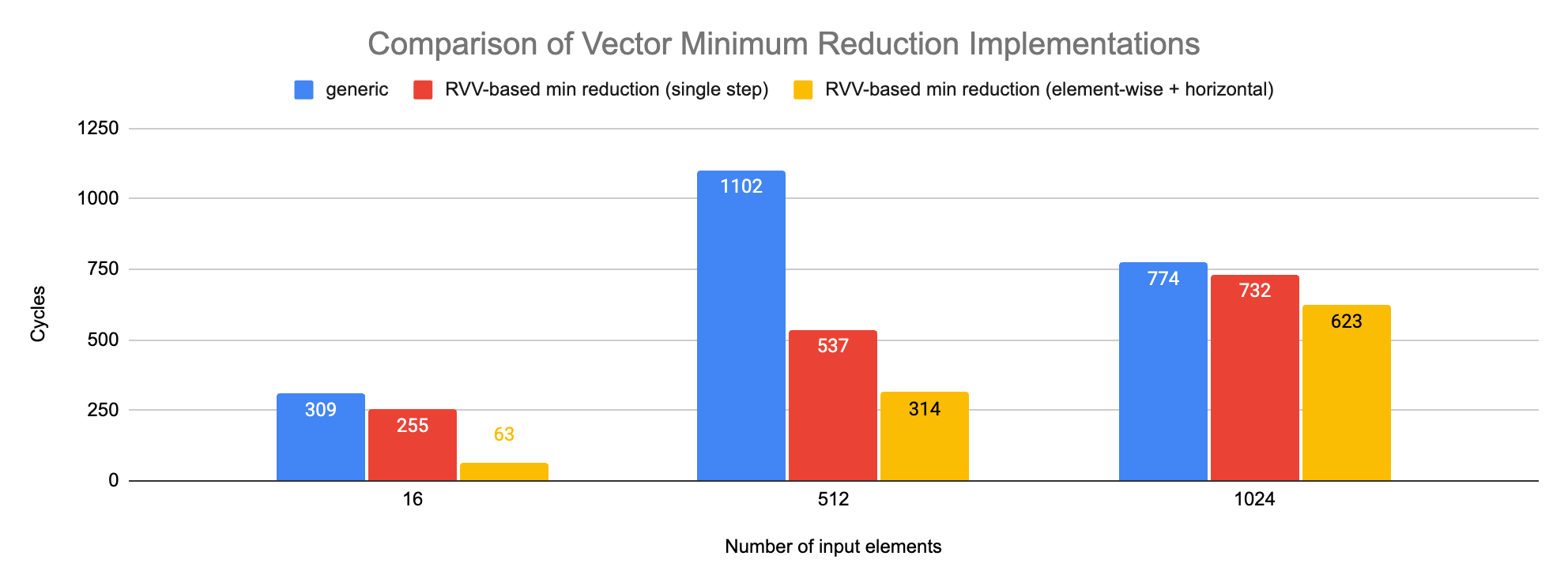
The implementation we described previous corresponds to the label “RVV-based min reduction (single step)”. The 2-step implementation (using element-wise for the loop and a single execution of the actual vredmin.vs for the epilog) provides the best result. The relative advantage decreases when the size of the input vector increases.

For 16-element, the element-wise + horizontal variant exposes a latency unexpectedly low. This artefact is only visible on LMUL=4 in my runs, other LMULs exhibit either a value much closer to the single step version.

The benchmarking results for vector dot product are represented below (vertical axis uses a logarithmic scale):

The snippet listed previously in this post, corresponds to the label “RVV (single step, ordered)”. The parallel accumulation + unordered version corresponds to the second variant presented in this post.

With larger vector sizes, we can see that the unordered FP reduction outperforms the ordered version. The parallel accumulation version outperform the 1-step versions based solely on reduction instructions.

Another interesting measurement is the synthetic latency of a few vector reduction instructions on that hardware platform. To perform this, we built a synthetic benchmark chaining 30 calls of the same instruction on the same data. We make an overall latency measurement and divide by the number of times the instruction is called. We make such measurement for each value of vl from 0 to vlmax.

The results are plotted below:

A few things we can note from those benchmarks on the K230:

• latency does not vary linearly with vl, it is rather constant, regardless of vl (even exhibiting a similar value when vl=0 !)

• vfredusum.vs is about twice as fast as vfredosum.vs

• Integer vredmin.vs and vredsum.vs latencies are quite similar (oscillating somewhere around 20 cycles per instruction regardless of the value of vl)

To understand what is going on, we can plot the latency for various values of LMUL and for similar vector lengths:

We can see that for a given LMUL value, latency is not really correlated with vl. And for the same vl, the latency increases with LMUL. The Kendryte K230 is definitely not optimizing reductions as much as it could !

Conclusion

Reduction operations are a necessary complement to element-wise operations in any SIMD Instruction Set Architecture. RISC-V Vector 1.0 offers quite a few different operations with some subtleties in particular with respect to floating-point sums . The extension does not force any specific scheme for the non-associative floating-point reduction sum and offer both an ordered scheme, amenable for C-like loop vectorization and an unordered scheme more lenient towards the implementation.

Reductions can be powerful operations but need to be implemented and use with care, in particular micro-architecture performance can vary widely on those instructions and a mix of element-wise and linear reduction operations may be required to get the best performance out of implementations (in particular on the low end).

Updated April 20th 2025: following some comments made by Al M., we have updated the unordered reduction illustration and added a paragraph to emphasize that floating-point addition is non-associative and this makes defining a unique result for a FP reduction sum impossible if an evaluation order is not defined.

Reference(s)

• RISC-V Vector specification: Vector Reduction Operations section

• camel-cdr
  benchmarked the K230 instruction (results here) and seems to have found similar latencies for the reduction instructions (as well as the dependency on VLMAX/LMUL rather than vl)

1. If you need a refresher on RVV you can check our series RVV In a Nutshell:

RISC-V Vector in a Nutshell