RVV implementation of Keccak / SHA-3 (part 1)

Leveraging RISC-V Vector to slow down SHA-3 software implementation

(Updated April 27th 2025: adding clearer diagram for χ step)

In this post we are going to study how to implement the SHA-3 Keccak round function using RISC-V Vector. The goal is to evaluate if the current RVV (+Zvbb) can provide speed-up over an optimized scalar implementation.

This post starts by an introduction to the Keccak algorithm, followed by a theoretical study of some ways it can be vectorized. Finally we evaluate the impact of vectorization through theoretical (retired instructions) and practical (latency on T-Head C908) benchmarkings. This post is the first one of a series reviewing multiple experiments around Keccak vectorization using RVV, as you will see at the end of this first post some efforts are still required to provide actual speedups.

Keccak in a nutshell

Keccak is the building block used in NIST SHA-3 hash function family. This highly configurable function (you can check the official summary for a more in-depth overview) is built around a multi-round permutation: Keccak-f. In the most used configuration, the permutation inputs and outputs a 1600-bit state. This state can be viewed as a 5x5 Matrix A of 64-bit elements¹. The permutation consists in multiple executions of a round function. The round function is built out of 5 steps labelled θ, ρ, π, χ, and ι. Here is the pseudo-codes (source) for Keccak-f and the round function (for the standard use SHA-3 and its extendable output counterpart SHAKE n=24):

# A[x, y] is a 64-bit lane with x in 0…4 and y in 0…4

Keccak-f[b](A) {
  for i in 0…n-1
    A = Round[b](A, RC[i])
  return A
}

Round[b](A,RC) {
  # θ step
  for x in 0…4
     C[x] = A[x,0] xor A[x,1] xor A[x,2] xor A[x,3] xor A[x,4],   

  for x in 0…4
     D[x] = C[x-1] xor rot(C[x+1],1), 

  for (x,y) in (0…4,0…4)
     A[x,y] = A[x,y] xor D[x],           

  # ρ and π steps
  for (x,y) in (0…4,0…4)
     B[y,2*x+3*y] = rot(A[x,y], r[x,y])                 

  # χ step
  for (x,y) in (0…4,0…4)
     A[x,y] = B[x,y] xor ((not B[x+1,y]) and B[x+2,y]),  

  # ι step
  A[0,0] = A[0,0] xor RC

  return A
}

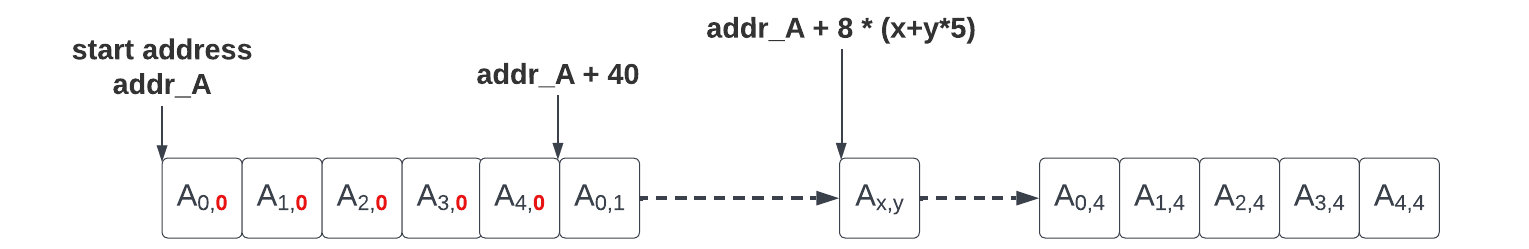
In the following we will assume that the state matrix A is initially stored in memory in a row-major layout: that is the y-th row, {A[0, y], A[1, y], A[2, y], A[3, y], A[4, y]}, is stored contiguously in memory starting from A[0, y], and the next row (if y < 4) starts in memory with A[0, y+1] appearing right after A[4, y] in increasing address order. At the end of the Keccak-f1600 function the resulting state must be stored back in memory with the same layout.

Let’s present each step before considering their vectorization.

θ step

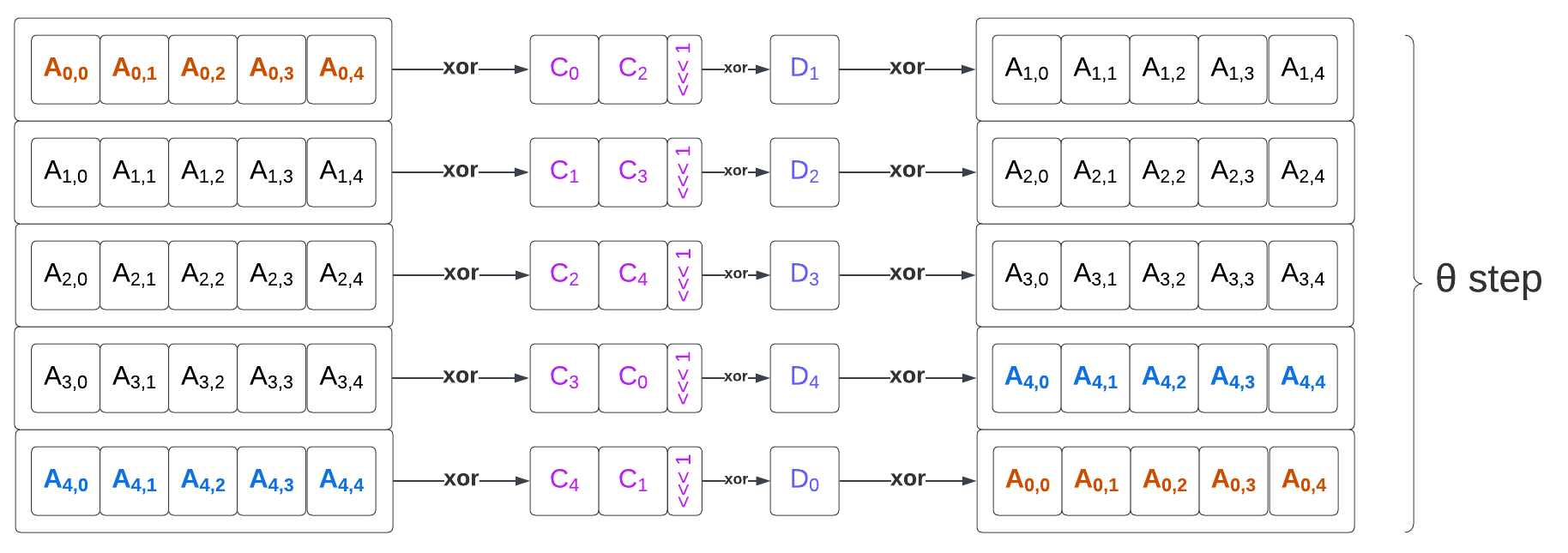
The θ step is made of 3 sub steps:

• Computing the parity vector C of each state column.

• Building the intermediary value D by XOR-ing the previous column and a 1-bit rotate of the next column value of C for each column.

• XOR-ing D with the whole initial A state (broadcasting values to the state columns).

The θ step performs 50 64-bit XOR operations and 5 64-bit left rotation operations (by one bit). The parity C computation exposes some data parallelism (XOR reduction can be evaluated with a binary tree) and XOR-ing D into A exposes 25 independent parallelizable operations.

ρ and π steps

# ρ and π steps
# r[x,y] is a 5x5 array of 25 constant rotation amounts
for (x,y) in (0…4,0…4)
   B[y,2*x+3*y] = rot(A[x,y], r[x,y])

The ρ is made of 25 64-bit rotations ,with a different rotation amount for each element.

The π steps is made of a 25-element permutation from the rotated values in A to the new state value B with source element x,y mapped to destination element y,2x+3y.

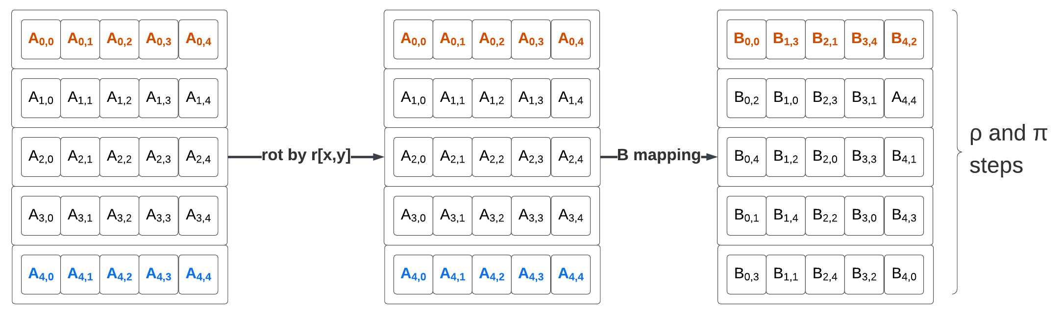
Rotation amounts are defined for each lanes, and the lane permutation from A to B is equivalent to a transpose followed by a per-column lane rotation. Before applying the per element rotation, the new mapping of A looks like this:

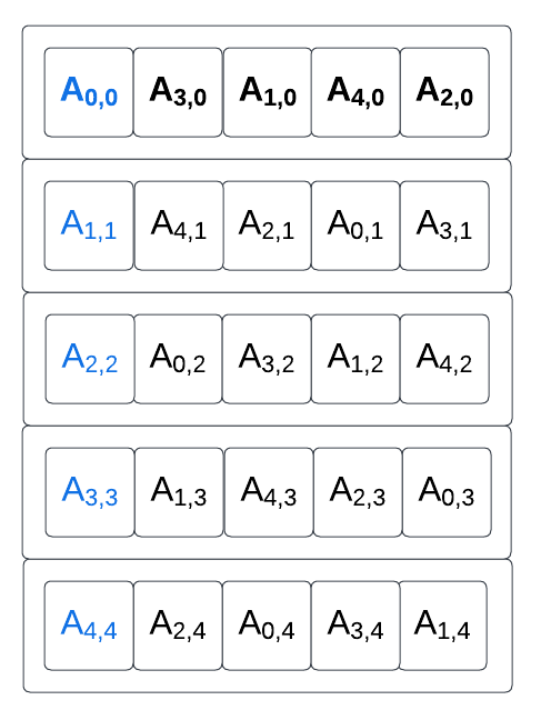
(A’s original diagonal is highlighted in blue and A’s original first column is highlighted in bold).

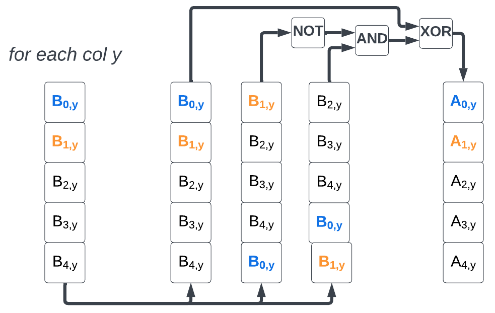
χ step

The χ step is made of 25 XOR, 25 NOT, and 25 AND operations. For each element, the operation inputs the current element, the next column element and the next-next column elements.

# χ step
for (x,y) in (0…4,0…4)
   A[x,y] = B[x,y] xor ((not B[x+1,y]) and B[x+2,y]),  

Note: In modern ISAs, the NOT and AND operations can often be fused in a single AND-NOT instruction. This is the case in RISC-V with the scalar andn instruction introduced in Zbb (and Zbkb) and with the vector vandn instruction introduced in Zvkb.

ι step

The ι step is simply a 64-bit XOR of the round constant into the first state lane. The round constant only depends on the value of i, the round index.

# ι step
A[0,0] = A[0,0] xor RC[i]

Scalar implementation of Keccak-f1600 round function

Overall an optimized implementation of Keccak would require around :

• 76 XOR operations (50 for θ, 25 for χ, 1 for ι)

• 30 rotation operations (5 for θ, 25 for π)

• 25 AND-NOT operations (χ step only)

In the github repository associated with this post you will find a first python script to generate an unrolled version of the scalar implementation for a round starting and ending with the state in memory. A second script generates a scalar implementation with input and output state in variables (more suitable for in-register code generation).

Vector implementation

For our vector implementation we start from the standard implementation from Keccak-readable-and-compact.c.

The full implementation (and the benchmark) can be found here. In this section we are going to review some of the details of the vectorization techniques we explored for our RVV based implementation.

In this experiment we chose to vectorize Keccak on a single state. This raises interesting challenges as the state permutation which is free when unrolling the scalar implementation (see for example this implementation) is no longer free with the vector implementation and must be actually performed if we want to pack multiple lanes together to try to exploit some of the data level parallelism exposed by the permutation function.

Storing the 1600-bit state: a group per lane

The 1600-bit state of Keccak is quite large. Assuming VLEN=128, it requires a total of 12.5 vector registers. In this first vectorization effort, we have chosen to organize it has 5 320-bit rows. Each row corresponds to 5 64-bit lane. On a VLEN=128 implementation, the 320-bit row can be loaded as a (partial) LMUL=4 vector register group, while wasting about 37.5% register space in the used groups.

Here is an example of how to load the 5 vector register groups (one per row):

vuint64m4_t row0 = __riscv_vle64_v_u64m4(((uint64_t*)state) + 0, 5);
vuint64m4_t row1 = __riscv_vle64_v_u64m4(((uint64_t*)state) + 5, 5);
vuint64m4_t row2 = __riscv_vle64_v_u64m4(((uint64_t*)state) + 10, 5);
vuint64m4_t row3 = __riscv_vle64_v_u64m4(((uint64_t*)state) + 15, 5);
vuint64m4_t row4 = __riscv_vle64_v_u64m4(((uint64_t*)state) + 20, 5);

This register storage layout allows to implement the start and end of the θ step (parity C evaluation and XOR-ing of D into the state) with wide vector operations.

Note: For VLEN=128 implementations, It would be interesting to evaluate a Keccak implementation which mixes LMUL=2 register groups and one single 64-bit scalar register or a LMUL=1 vector register to store the 320-bit rows (reducing storage waste to either 0 or about 17%). Using a LMUL=4 vector register group, although wasting vector architectural registers is quite efficient in term of number of instructions required to perform the Keccak-f round.

Another solution would be to pack multiple 5-element rows into the same vector register group with or without overlap:

• (A) Packing 15 elements from rows 0, 1, and 2 into a 16-element LMUL=8 vector register group and packing 10 elements from rows 2 and 3 into another groups (no overlap)

• (B) Packing 16 elements from rows 0, 1, 2, and 3 into a 16-element LMUL=8 vector register group (with only the least significant element from row 3 appearing as the group most significant element) and packing 9 elements from row 2 and 3 into another groups (keeping only the 4 most significant elements from row 2).

Vectorizing the θ step

With our chosen register layout vectorizing two out of the 3 sub-steps of the θ step is rather easy. The parity vector C can be evaluated in parallel for each column:

vuint64m4_t C_01  = __riscv_vxor_vv_u64m4(row0, row1, 5);
vuint64m4_t C_23  = __riscv_vxor_vv_u64m4(row2, row3, 5);
vuint64m4_t C_014 = __riscv_vxor_vv_u64m4(C_01, row4, 5);
vuint64m4_t C     = __riscv_vxor_vv_u64m4(C_23, C_014, 5);

Computing the D vector requires some permutations to obtain rotated versions of C. We compute D_opHi correspoding to C[x-1]:

// {C[4]}
vuint64m4_t C_4_ext = __riscv_vslidedown_vx_u64m4(C_vector, 4, 1);
// {C[4],    C[0], C[1], C[2], C[3]}
vuint64m4_t D_opHi = __riscv_vslideup_vx_u64m4(C_4_ext, C_vector, 1, 5); 

Note: The intrinsics is called __riscv_vslideup_vx but it will actually be implemented by a vslideup.vi since the slide amount is an immediate constant (there is not a specific intrinsic for the latter).

Note: We exploit the fact that RVV’s vslideup.vi maintains unmodified the elements whose index is lower than the slide amount to perform the element rotation by a vslidedown.vi followed by a vslideup.vi.

We also compute D_opLo correspoding to rot(C[x+1],1) and we XOR it with D_opHi:

// {C[1], C[2], C[3], C[4], 0}
vuint64m4_t D_opLo = __riscv_vslidedown_vx_u64m4(C_vector, 1, 5);
// {C[1], C[2], C[3], C[4], C[0]}
D_opLo = __riscv_vslideup_vx_u64m4(D_opLo, C_vector, 4, 5);
D_opLo = __riscv_vrol_vx_u64m4(D_opLo, 1, 5);
vuint64m4_t D = __riscv_vxor_vv_u64m4(D_opLo, D_opHi, 5);

D’s layout is compatible with a direct element-wise XOR-ing with each rows:

row0 = __riscv_vxor_vv_u64m4(row0, D, 5);
row1 = __riscv_vxor_vv_u64m4(row1, D, 5);
row2 = __riscv_vxor_vv_u64m4(row2, D, 5);
row3 = __riscv_vxor_vv_u64m4(row3, D, 5);
row4 = __riscv_vxor_vv_u64m4(row4, D, 5);

Vectorizing ρ and π steps

ρ and π steps are built from a permutation from matrix A to matrix B and bit rotations for each element of B (with non-uniform rotation amounts).

There are multiple ways to implement the permutation from A to B: using indexed loads (or store), using vrgather …

We rely on a reverse mapping to evaluate the source for B[i,j]: i=y, j=2*x+3*y thus y=i, 2*x=(j-3*y).

Variant 1 for ρ and π steps: using indexed memory access

The first technique to perform the ρ and π steps is to use a vector (unordered) indexed load: vluxei16. A static array containing in order the byte offset for each element of B is used as the index source. Another static array stores the bit rotation amount to be applied to each element of B.

The full B array is processed in two steps using LMUL=8: the first step performs ρ and π on the first 16 elements of B while the second step performs ρ and π on the last 9 elements.

uint16_t offset_AtoB[] = {
    // byte offset for each index
    0, 48, 96, 144, 192, 
    24, 72, 80, 128, 176, 
    8, 56, 104, 152, 160, 
    32, 40, 88, 136, 184, 
    16, 64, 112, 120, 168, 
};
uint64_t rotation_B[] = {
    0, 44, 43, 21, 14, 
    28, 20, 3, 45, 61, 
    1, 6, 25, 8, 18, 
    27, 36, 10, 15, 56, 
    62, 55, 39, 41, 2, 
};

// The following assumes VLEN >= 128, and uses 2x 8-register groups to load/transpose 
// matrix A to B
// First 16 elements [0...15]
// loading the byte offsets for A to B
vuint16m2_t B_index_0 = __riscv_vle16_v_u16m2(offset_AtoB, 16);
// using the byte offsets to address A and extract the first 16 elements
vuint64m8_t B_0 = __riscv_vluxei16_v_u64m8(state, B_index_0, 16);

// loading the rotation amounts for the first 16 elements
vuint64m8_t B_rots_0 = __riscv_vle64_v_u64m8(rotation_B, 16);
// applying the rotations to the first 16 elements
B_0 = __riscv_vrol_vv_u64m8(B_0, B_rots_0, 16);

// Last 9 elements [16...24]
(...)

Note: there is no constraint on the ordering of element accesses in the indexed load execution. Thus the unordered variant vluxei* can be selected over the ordered variant vloxei*: the former leave more room for micro-architectural optimization and could be faster on some implementations.

Note: we have presented an implementation with indexed load; an implementation with indexed store is possible assuming the state is expected in memory after the execution of the ρ and π steps. The element rotations would have to be performed on the un-permutated A matrix before the store.

Variant 2 for ρ and π steps: using in-register vrgather(ei16)

The second vectorization variant for the ρ and π steps is to use in-register permutation.

As described the θ step, we have chosen to store each state row in a different vector register group. In step π, each row of B receives elements from all the rows of A. So a solution to avoid indexed load in memory is to build a very large in-register input data set and use it to generate each destination row.

Since we chose to focus on implementations compatible with VLEN=128, the largest state we can have is a LMUL=8 vector register group containing 16 elements. It is not enough to cover the 25 elements in a Keccak state; this means we need at least two such data sets to cover the full input state.

Here is how we build those input data sets, rho_data_lo and rho_data_hi:

// building two input sets
// first set {row0[0..4], row1[0..4], row2[0..4], 0}
row0 = __riscv_vslideup_vx_u64m4(row0, row1, 5, 8);
row1 = __riscv_vslidedown_vx_u64m4(row1, 3, 3);
row2 = __riscv_vslideup_vx_u64m4(row1, row2, 2, 8);
vuint64m8_t rho_data_lo = __riscv_vcreate_v_u64m4_u64m8(row0, row2);

// second set {row3[0..4], 0, 0, 0, row4[0..4], 0, 0, 0}
vuint64m8_t rho_data_hi = __riscv_vcreate_v_u64m4_u64m8(row3, row4);

and then we build two sets of indices to address the input data sets:

// index for each row (5-element) in rho_data_lo
// Note: -1 value triggers an index overflow in vrgather(ei16)
// the corresponding result element with be filled with 0s.
const uint16_t offsetIndex_AtoB_lo[] = {
    // index offset for each index
    0, 6, 12, -1, -1, 
    3, 9, 10, -1, -1, 
    1, 7, 13, -1, -1, 
    4, 5, 11, -1, -1, 
    2, 8, 14, -1, -1, 
};
// Index array for each row (5-element) in rho_data_hi.
// The indices are offset to index in rho_data_hi by subtracting
// 15 from their values used in indexed loads.
// Elements which were extracted from rho_data_lo are indexed by -1 to
// be filled with 0s (compatible with OR-ing with the
// result of the first indexing) 
const uint16_t offsetIndex_AtoB_hi[] = {
    // index offset for each index
    -1, -1, -1, 18 - 15, 24 - 20 + 8, 
    -1, -1, -1, 16 - 15, 22 - 20 + 8, 
    -1, -1, -1, 19 - 15, 20 - 20 + 8, 
    -1, -1, -1, 17 - 15, 23 - 20 + 8, 
    -1, -1, -1, 15 - 15, 21 - 20 + 8, 
};

Finally we construct B, row by row, by indexing into rho_data_lo and rho_data_hi and then combining (OR-ing) the results. For example, for the first row, the code might look like:

vuint16m2_t B_index_row0_lo, B_index_row0_hi;

// loading indices
B_index_row_lo  = __riscv_vle16_v_u16m2(offsetIndex_AtoB_lo, 5);
B_index_row0_hi = __riscv_vle16_v_u16m2(offsetIndex_AtoB_hi, 5);

// indexing the two in-register data sets and combining the results
row0 = __riscv_vor_vv_u64m4(
  __riscv_vget_v_u64m8_u64m4(__riscv_vrgatherei16_vv_u64m8(rho_data_lo, B_index_row0_lo, 5), 0),
  __riscv_vget_v_u64m8_u64m4(__riscv_vrgatherei16_vv_u64m8(rho_data_hi, B_index_row0_hi, 5), 0),
  5
);

// per-element rotations (pi step)
// loading per element rotation amounts
vuint64m4_t B_rots_row0 = __riscv_vle64_v_u64m4(rotation_B + 0 * 5, 5);
// applying per elemen rotations
row0 = __riscv_vrol_vv_u64m4(row0, B_rots_row0, 5);

χ step and ι step

For the χ step, we can leverage the vector instruction vandn.vv introduced in the vector crypto Zvkb extension. This instruction fuses the two vector operations v not.v and vand.vv.

To vectorize the χ step, we need to rotate B’s rows before applying the vector XOR and vector AND-NOT operations.

foreach row from B{
  // {row[1], row[2], row[3], row{4}}
  vuint64m4_t row_xp1 = __riscv_vslidedown_vx_u64m4(row, 1, 4);
  // {row[2], row[3], row[4]}
  vuint64m4_t row_xp2 = __riscv_vslidedown_vx_u64m4(row, 2, 3);

  // {row[1], row[2], row[3], row[4], row[0]}
  row_xp1 = __riscv_vslideup_vx_u64m4(row_xp1, row, 4, 5);
  // {row[2], row[3], row[4], row[0], row[1]}
  row_xp2 = __riscv_vslideup_vx_u64m4(row_xp2, row, 3, 5);

  vuint64m4_t vandn = __riscv_vandn_vv_u64m4(row_xp2, row_xp1, 5);
  row = __riscv_vxor_vv_u64m4(row, vandn, 5);
}

The ι step being a single 64-bit XOR, it can be merged with the χ step and performed with a simple vxor.vv with vl=1 and tail agnostic policy:

if (rowId == 0) row = __riscv_vxor_vx_u64m4_tu(row, row, RC[round], 1);

Benchmarks

We are going to use Keccak-compact-test.c from XKCP as our test.

We are going to bench the KeccakF1600 function (which executes 24 Keccak rounds), and from this measurement we will also report approximate instruction counts for a single Keccak round. By “benchmark” we actually mean counting the number of retired instructions. This metric is usually not a good proxy for actual program performance (since different instructions can expose different latencies, with potentially large variabilities and dependence on the micro-architecture, especially when memory and vectors are involved). We consider this sufficient for this exercise (do not use the implementation with the least amount of executed instructions and expect it to be the fastest).

We built each implementation using clang/llvm version

clang version 18.0.0git (https://github.com/llvm/llvm-project.git 5cfc7b3342ce4de0bbe182b38baa8a71fc83f8f8)

with the following options:

--target=riscv64 \
-O3 \
-menable-experimental-extensions \
-march=rv64gcv_zvbb1p0_zbb_zbc_zba

Note: enabling bit manipulation ISA extensions (in particular Zbb and Zvbb / Zvkb) is key to Keccak performance since the algorithm relies heavily on bit rotations and AND-NOT which are not part of RISC-V base ISA or base Vector extension.

Benchmarking scalar implementations

The first implementation to be measured is from Keccak-more-compact.c. This is a simple and compact implementation.

The second implementation is from Keccak-readable-and-compact.c. This is a more readable version of the Keccak implementation. We built it with the same compiler version and same options.

These baseline scalar implementations are far from the expected performance of a Keccak round. As we have seen earlier in this post, discounting memory access, the Keccak round requires about 155 operations, so we should be able to execute it with a number of instructions in that ball park. To get closer to that mark, we developed an unrolled version (source code) which try to access memory only when loading and storing the state before and after executing the 24 rounds (Our C-based implementation still do some spilling). With this implementation we get about 176 instructions retired to execute a single KeccakF1600 round. We also bench a scalar unrolled version which does not try to avoid memory accesses.

Benchmarking vector implementations

The next implementation is our first vectorized version (source code), then we bench a vector-in-reg version which implements the ρ and π steps using in-register permutes. Finally, we implement a vectorized multi-round version, closer to the first version but which maintain the state in register between two rounds (while still relying on memory round-trip for ρ and π steps).

Results

The reported results are an average of the the number of retired instruction per Keccak rounds during runs of SHA3-224 on riscv-isa-sim (spike) simulator. The benchmark consists in 5193 calls to KeccakF1600_StatePermute or 124632 KeccakF1600 rounds.

testKeccakInstanceByteLevel(1152,
                            448,
                            0x06,
                            28,
                            "\xf3\x61\xcb\xd5\x9b\x84\x1d\x8e\x0c\xdb"
                            "\xd4\x06\x1e\xb5\x7a\xea\x75\x1d"
                            "\x34\x36\x01\x23\x6e\xef\x0c"
                            "\x5d\x81\x7b"); /* SHA3-224 */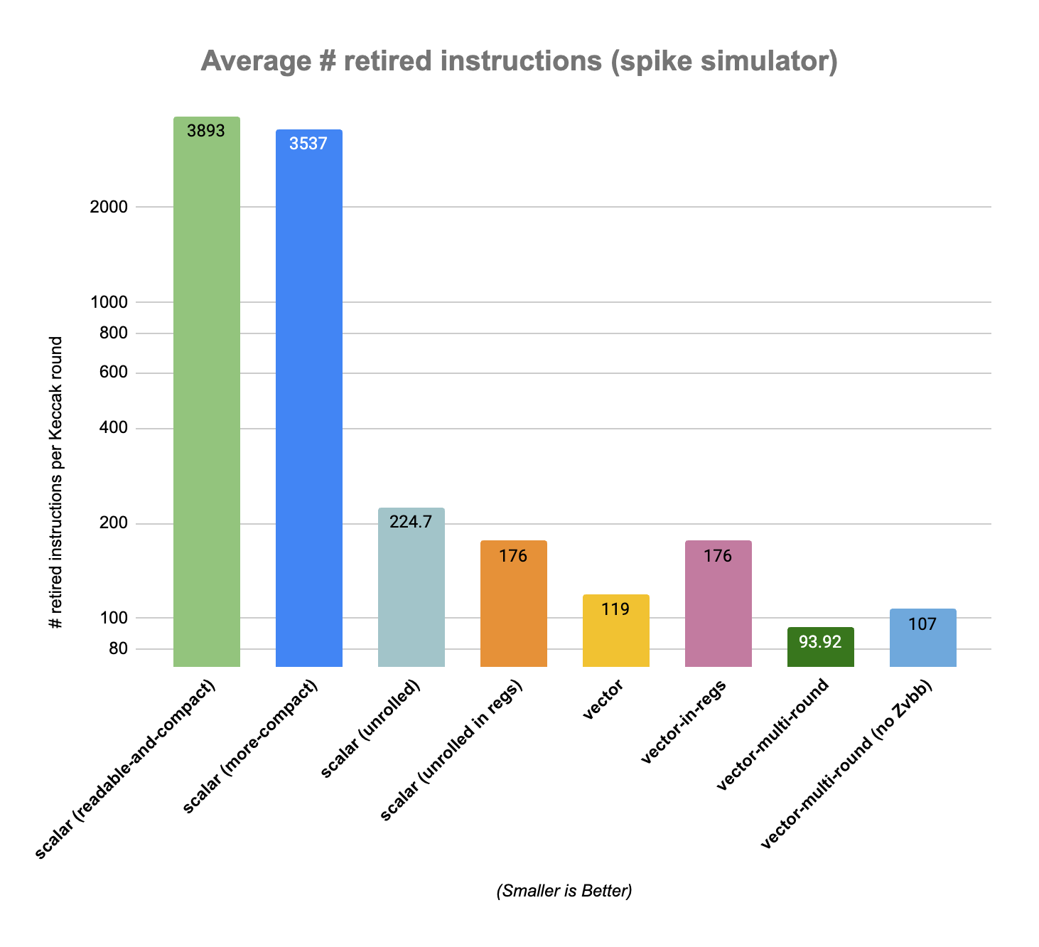

Note: we also benchmarked a multi-round vectorized version without enabling Zvbb, the vector basic bit manipulation extensions. This version requires about 14% more instructions to perform a Keccak round than the version with Zvbb enabled (107 retired instructions per round versus 94).

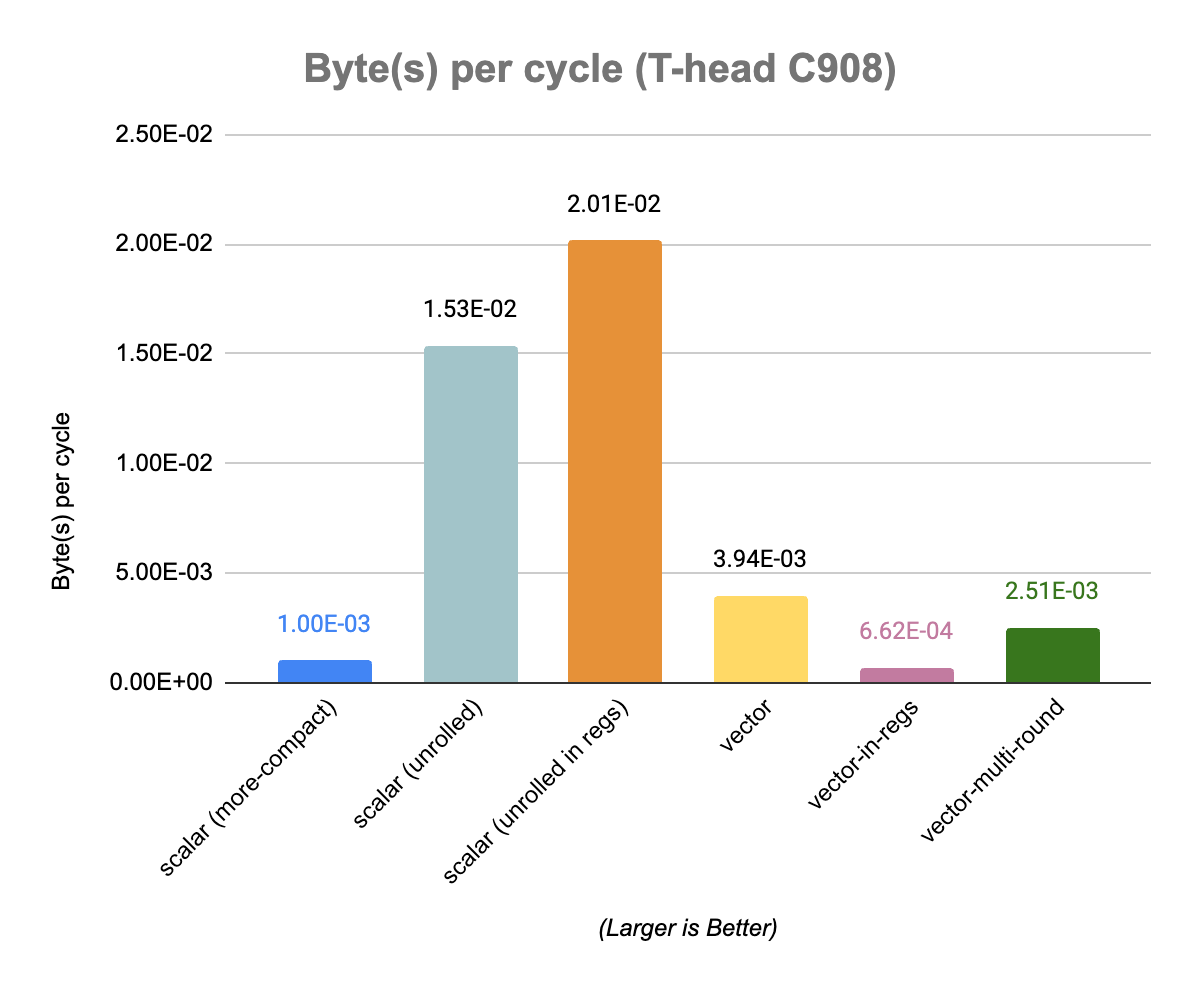
Actual benchmarks on a hardware platform (T-Head C908) done by Camel Coder reveal abysmal performance for the vector implementations (more details here). As expected the number of retired instructions does not convert into a similar behavior when it comes to the actual execution latency. The best scalar implementation, unrolled-in-regs, clocks at about 0.02 Byte per cycle, while the best vector implementation, the baseline vector implementation, is about 5 times slower at around 0.004 Byte per cycle (Camel’s full results and analysis can be found on the github issue). The C908 seems to have a limited width vector datapath which makes running vector code on larger element width not really competitive against scalar execution. In addition some of the more complex vector operations used by our implementations exhibit a low throughput.

Conclusion

Keccak vectorization has a very large solution space and not all of them lead to efficient implementation. One of the challenge is that some of the static permutations part of a KeccakF1600 round, which were no-operation in optimized scalar implementations, have become actual vector operations (e.g. permutation of the π step) and they map to generally slow instructions in vector processors (indexed load/store or vrgather).

Using RVV to accelerate multiple Keccak evaluations in parallel seems more promising. We will explore this and revisit the vectorization of the Keccak permutation function in a future to try to improve our current results. It will also be interesting to measure how the optimized scalar and vector implementation behave on a more performant out-of-order RISC-V implementation. There is also some litterature on extending RISC-V Vector for better SHA-3 support that I would like to review and that is being considered in RISC-V Post Quantum Cryptography task group (SHA-3 being one of the key component in some of the newly specified PQC algorithms, in particular for deterministic asset generation from keys).

Thank you to Camel Coder for running the code on an actual hardware platform and providing actual latency results.

References

• https://keccak.team/keccak_specs_summary.html

• https://github.com/XKCP/XKCP/tree/master/Standalone/CompactFIPS202/C

• https://github.com/nibrunieAtSi5/rvv-keccak/tree/main

• https://github.com/XKCP/XKCP/tree/master/lib/low/KeccakP-1600-times2/SIMD128

• RISC-V blog post on T-Head C908: https://riscv.org/blog/2022/11/xuantie-c908-high-performance-risc-v-processor-catered-to-aiot-industry-chang-liu-alibaba-cloud/

• Maximizing the Potential of Custom RISC-V Vector Extensions for Speeding up SHA-3 Hash Functions, Huimin Li and al. (https://eprint.iacr.org/2022/868) [study of ISA extensions to speed-up SHA-3 on RISC-V]

1. Other Keccak configurations exist for different word sizes (e.g. 32-bit).