Number Theoretic Transform with RVV

It is all about computing in the right space (and using cheap transforms)

Numerous modern cryptographic algorithms rely on multiplications of large polynomials (e.g. Post Quantum Cryptography and Fully Homomorphic Encryption algorithms based on the Learning With Error [LWE] problem). Computing such multiplications is computationally expensive and often represents a large part of the overall complexity of the algorithm.

The Number Theoretic Transform, or NTT, is a well known method to rapidly multiply two polynomials. It corresponds to the application of the Fourier transform on polynomial rings. It can benefit from the same fast evaluation techniques as the ones usually exploited to implement Fast Fourier Transform (FFT). For large degree polynomials, when the cost of the transform can be amortized, it offers very interesting speed-up versus naive multiplication implementations (and the polynomial modulo reduction comes for free as part of the transform).

In this post we will survey the basis of polynomial multiplication, review the NTT method and present an implementation using RISC-V Vector. The literature on FFT and NTT is quite extensive, and lots of effort have been made to optimize the implementation of those algorithms, we will only scratch the surface of those techniques but this should still be an interesting journey.

Multiplication of polynomials

We are considering the multiplication of two degree n polynomials: L (coefficients Li) and R (coefficients Ri). Coefficients are integers with values in Zq: every operations on coefficients is performed modulo the integer q. In the cases that interest us, q is prime and Zq is a field.

The polynomial multiplication is evaluated modulo a third polynomial M whose degree is n+1. We only consider the case where the most significant coefficient of M is 1 (this aligns with the values used in practice).

\((L_0 + L_1 . X + ... L_n . X^n) \times (R_0 + ... R_n . X^n)~ mod ~(M_0 + M_1 . X + ... + X^{n+1})\)

Note: In the applications of interest M is a polynomial with very few non-zero coefficients. Thus we could even restrict ourselves to cases where all the other coefficients of M are 0, except the most significant coefficient (which is 1), and the least significant coefficient M0 which is either 1 or -1.

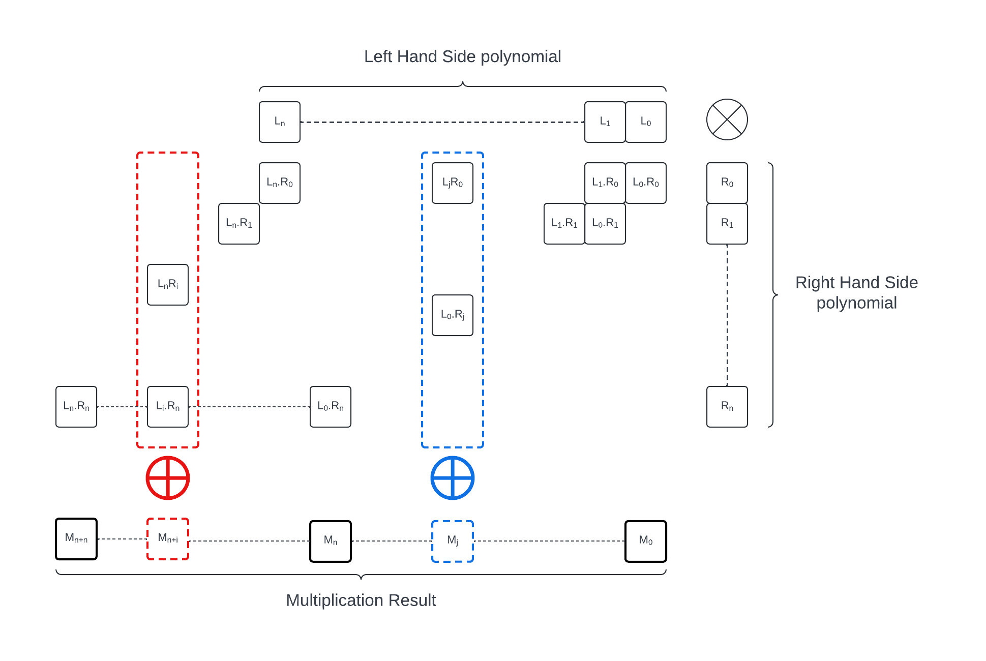
A dummy method for polynomial multiplication is illustrated below. It scans through the monomial Ri of the polynomial R and multiplies each of them by L, accumulating the result: every Li.Rj with i+j=d must be accumulated in the resulting coefficient of index d. This algorithm requires (n+1)^2 multiplications in Zq and O(n^2) additions.

The result needs to be reduced modulo M. In our case, since the most significant coefficient of M is 1, this can be easily implemented: we perform the multiplication starting with the most significant coefficient or R. and compute:

\(A = R_n \times L\)

This is at most a degree n polynomial. In the second step we compute:

\( A = R_n.L.X + R_{n-1}.L \)

This is at most a degree n+1 polynomial. We reduce it modulo M by performing

\(A = A - A_{n+1} \times M\)

and we get back a polynomial of degree at most n. We iterate over the coefficients of R as follows:

\(A = (A \times X - A_n \times M) + R_i \times L \)

until the last step:

\(A = (A \times X - A_n \times M) + R_0 \times L \)

which provides the multiplication modulo M result.

In each iteration we can skip the computation of the coefficient of degree n+1: A_n.M_{n+1} = A_n will always cancel out the most significant coefficient of A.X. Overall the modulo reduction steps adds at most n coefficient multiplications and n coefficient subtractions per iteration (so O(n^2) total operations). In the real application case M has a constant number of non-zero coefficients (generally 1, excluding the most significant one) and so the modulo reduction can be done in O(n) operations.

Modulo arithmetic for coefficients

Integer arithmetic modulo q is expansive when it is implemented using a complete remainder operation. This can easily be avoided for addition (by subtracting the modulo if the addition result exceeds it) but requires more “advanced” techniques when it comes to multiplication.

For this, we will exploit Barrett’s modular reduction method.

Let’s exemplify it with a modulo q=3329 (modulo used for Kyber). We introduce m=2^k/q and m’=floor(2^k/q)=5029, for k=24 (twice the bit size of the modulo).

Assuming a value a, we compute a - ((m’ * a) » k) * q, this value is within [0, 2*q[ so a subtraction of q might be required when it is within the subset [q, 2q[.

To make this scheme more amenable to a vector implementation, we can used signed arithmetic and compute m’’=ceil(2^k/q), a-((m’*a)»k)*q is now within [-q, q[ and addition of q might be required. This addition needs to be perform if the initial value is negative; a mask should easily be buildable for this predicate and applied to condition the addition.

Note: Using Barrett’s algorithm rather than a remainder operation can help implementation constant latency routines (or at least routines whose latency is independent from the data values). This applies to other part of the implementation and control flow and masking application should be made carefully to ensure the execution latency does not depend on the mask value.

The use of Barrett’s algorithm can certainly accelerate the polynomial multiplication but it does not reduce its theoretical complexity: if the dummy algorithm is used, this is still an operation with quadratic complexity in the size of the polynomial: we have just made the coefficient arithmetic faster on most implementations.

Introduction to Number Theoretic Transform

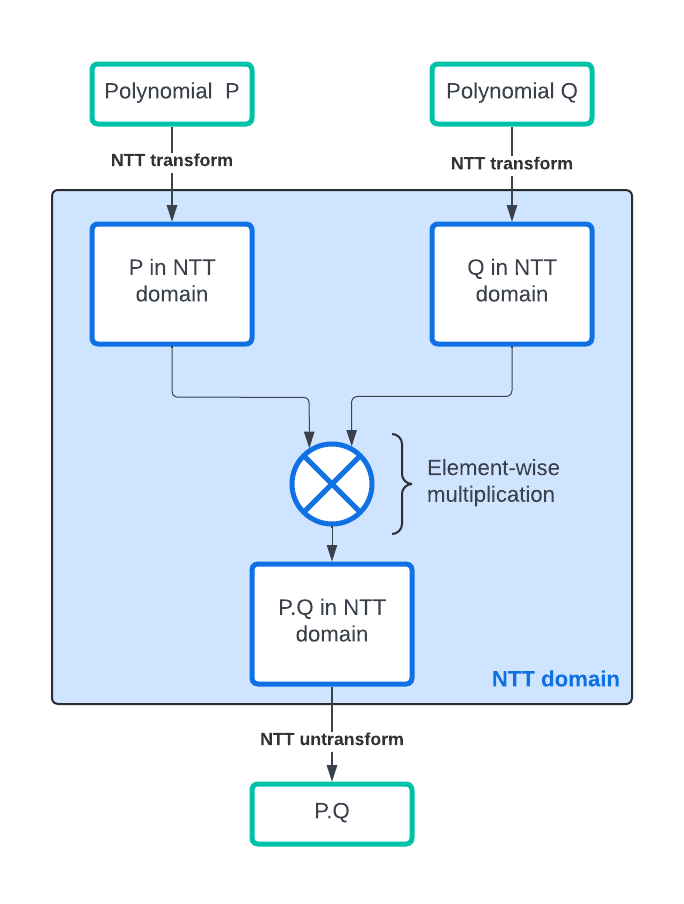
Number Theoretic Transform (or NTT) is the application of the Fourrier Transform to Polynomial Rings. Rather than evaluating the polynomial multiplication on the canonical form as described previously, we first transform each operand into the NTT domain, we then perform the multiplication operation in the NTT domain and finally we transform back the result into the canonical domain. The speed-up obtained from this method comes from the fact that transform and inverse transform can be evaluated very rapidly as they boast a O(n.log(n)) complexity with n the number of polynomial coefficients using an algorithm derived from the Fast Fourrier Transform algorithm; and the multiplication in the NTT domain can be performed in O(n) operations.

For a more in-depth and accurate explanation, I recommend this blog post by Amber Sprenkels https://electricdusk.com/ntt.html.

An intuitive way to understand NTT is to consider a vector A of values in Zq: A=(a_0, a_1, a_2, …, a_n). If we evaluate the polynomials L and R on this vector, we get two vectors L(A) = (L(a_0), L(a_1), L(a_2), …, L(a_n)) and R(A) = (R(a_0), R(a_1), R(a_2), …, R(a_n)). Trivially (L * R)(A) = (L(a_0) * R(a_0), L(a_1) * R(a_1), L(a_2) * R(a_2), …, L(a_n) * R(a_n)) is the element-wise multiplication of the two vectors. If from L (respectively R) we can build L(A) (resp. R(A) efficiently, and from (L*R)(A) we can reconstruct (L*R) efficiently, then we can “efficiently” compute the multiplication L*R by evaluating both polynomials on the vector A, multiplying the results element-wise and then reconstructing the corresponding result polynomial. For a polynomial P, we call P(A) the representation in the NTT domain of P.

Definition of the NTT

NTT uses a principal n-th root of unity to build the vector A, let’s call it α. α verifies:

(Source: Wikipedia's article: Discrete Fourier transform over a ring)

the vector A is defined as:

\(1, \alpha, \alpha^2, .... \alpha^{n-1}\)

and P(A) becomes:

\(P(A) = (P(1), P(\alpha), ..., P(\alpha^i), ... P(\alpha^{n-1}) \)

with

\(P(\alpha^i) = \sum_{k=0}^{n-1}p_i.\alpha^{i.k}\)

Note that up to this point, we have not improve the polynomial multiplication complexity. transforming P into P(A) with the trivial methods requires O(n^2) operations (not an improvement compared to multiplying two polynomial directly).

Fast Number Theoretic Transform

NTT has the Fourrier Transform is suitable to fast algorithm. We are going to use of the possible fast algorithm. If you’d like a more comprehensive survey, you can read one of the reference for this post: Number Theoretic Transform and Its Applications in Lattice-based Cryptosystems: A Survey,.

One of the fast way to evaluate the NTT transform is to used a version of the Cooley-Tukey algorithm: it relies on splitting the computation of each NTT coefficient into odd (O) and even (E) parts (for the Radix-2 version we consider, assuming n is even):

\(P(\alpha^i) = \sum_{k=0}^{n-1}p_k.\alpha^{i.k} = \sum_{k=0}^{\frac{n-1}{2}}p_{2k}.\alpha^{i.2k} + \sum_{k=0}^{\frac{n-1}{2}}p_{2k+1}.\alpha^{i.(2k+1)}\)

The odd/even split can be rewritten into:

\(P(\alpha^i) = \sum_{k=0}^{\frac{n-1}{2}}p_{2k}.(\alpha^{2i})^{k} + \sum_{k=0}^{\frac{n-1}{2}}p_{2k+1}.(\alpha^{2i})^{k}.\alpha^i\)

and finally:

\(P(\alpha^i) = E_i + \alpha^i.O_i = E(\alpha^{2i}) + \alpha^i . O(\alpha^{2i}) \)

E_i and O_i can be recursively evaluated as (n/2)-element NTTs with the root α^2.

The key element is that we can evaluate another coefficient using E_i and O_i:

\(P(\alpha^{i+\frac{n}{2}}) = \sum_{k=0}^{\frac{n-1}{2}}p_{2k}.\alpha^{(i+\frac{n}{2}).2k} + \sum_{k=0}^{\frac{n-1}{2}}p_{2k+1}.\alpha^{(i+\frac{n}{2}).(2k+1)}\)

This expression can be expanded into:

\(P(\alpha^{i+n/2}) = \sum_{k=0}^{\frac{n-1}{2}}p_{2k}.\alpha^{i.2k}.\alpha^{n.k} + \alpha^{i+\frac{n}{2}} . \sum_{k=0}^{\frac{n-1}{2}}p_{2k+1}.\alpha^{i.(2k)}.\alpha^{n.k}\)

And by exploiting the root of unity properties:

\(\alpha^{kn} = (\alpha^{n})^k = 1^k = 1, \ and \ \alpha^{\frac{n}{2}} = -1 \ (in \ \mathbb{Z}_q)\)

We get

\(P(\alpha^{i+n/2}) = E_i - \alpha^i O_i \)

So computing E_i and O_i allows us to get two NTT coefficients with an extra scalar multiplication by a power of the root of unity (sometimes referred to as twiddle factor), one addition and one subtraction. E_i and O_i are each n/2 element NTTs.

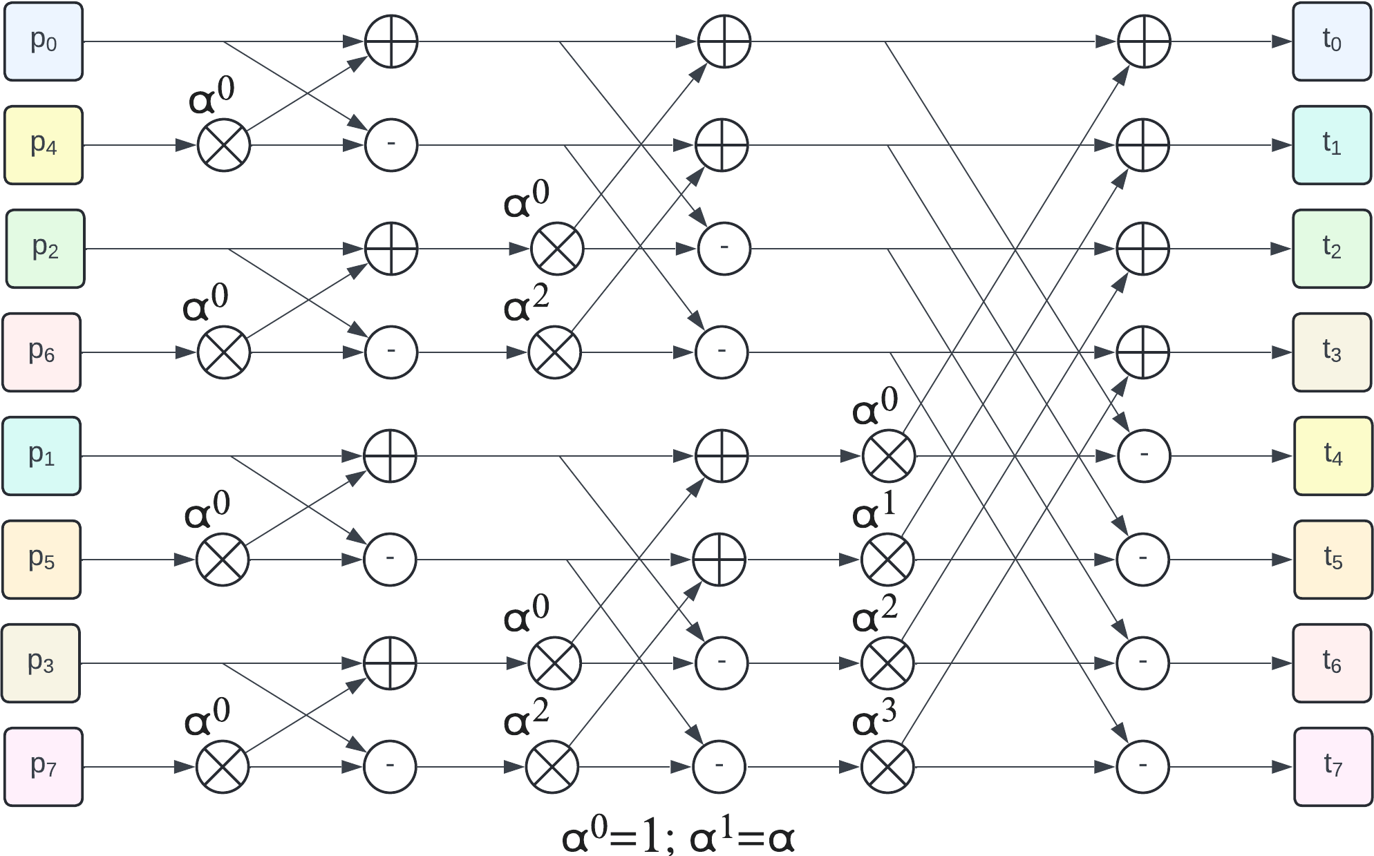
The recursive process of even/odd split followed by recursion is illustrated by the following figure (example for 8 elements):

8-coefficient Radix-2 Fast Number Theoretic Transform with α (8-th root of unity)

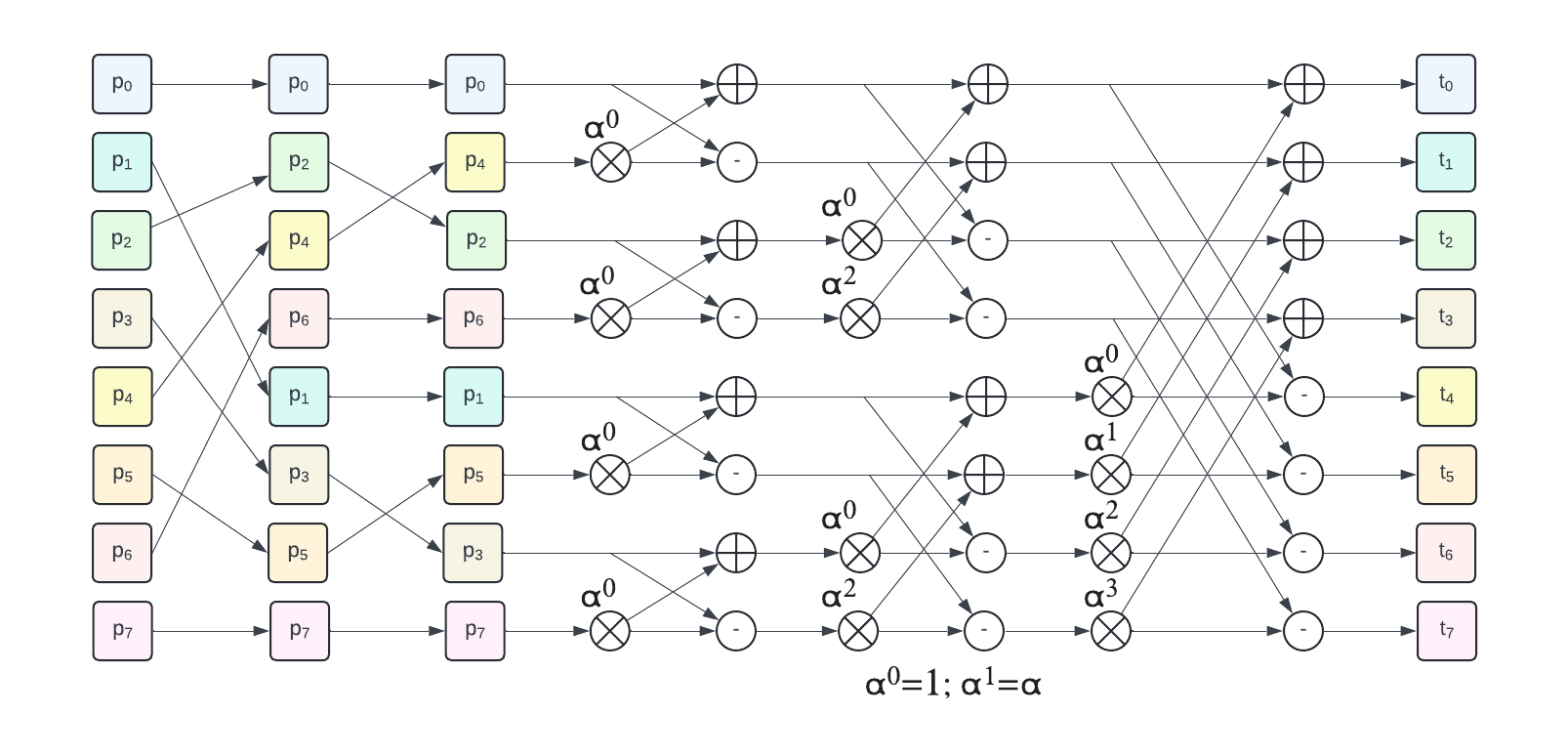
The 3 left hand side colored columns represent the recursive odd/even split. They are followed by 3 butterfly stages, the first one operates on 2-element groups, then 4-element groups and a final one on a single 8-element group to get the final NTT result.

This is but one of the many FFT/NTT techniques which exist.

Note: the techniques described in this post do not directly apply to Kyber because of some of the property of its NTT space: namely the fact that it uses 256-coefficient polynomial with a 256th root but no 512th root of unity and a X^n - 1 quotient polynomial.

NTT transform using RVV

Now that we have a fast algorithm, let’s consider how we can implement using RISC-V Vector. Our overall goal is to leverage the vector operations, single instruction multiple data paradigm, to accelerate the polynomial multiplication compared to a pure scalar implementation. There is a lot of parallelism in NTT computation but it does not always exposed a regular linear structure suitable for a straightforward mapping to vector operation.

The conversion from and to NTT domain requires a “somewhat” random addressing of elements. “somewhat” because it is not actually random (since it implements the well-known multi-level butterfly pattern ) but it requires gathering elements which do not fit a trivial access pattern.

The first implementation I selected to experiment with is a 2-stage process: we first permute the coefficients to get an array laying out the coefficients in such a way that at least one of the two coefficients of any butterfly stage is at the right index already.

There are a lot of optimizations that can be done.

We will first review how to perform the permutations by looking into two techniques: stage-by-stage permutations relying on unit or strided accesses and secondly performing the permutations in a single pass using a vector gather (from memory) instruction.

Stage by stage coefficient permutation

At each stage of the forward NTT step, the number of coefficients of each sub-NTT is divided by 2 compared to the previous stage.

The dummy RVV-based implementation is built around a 2-level loop: the outer level iterates on the stage levels and the second level iterates on each sub-NTT within that stage. At some points the sub-NTTs become very small and iterating over them is not an efficient use of vectors (e.g. a VLEN=128-bit datapath is not used to its plain potential if it only performs a single pair swap of 32-bit element for the last level butterfly). At those stages, it becomes interesting to fuse multiple sub-NTTs of the same stage together.

One of the benefit is that wider vectors can be used since multiple contiguous sub-NTT are fused together.

The following diagram illustrates how two 4-element sub-NTTs are fused together in two vector instructions operating on 8-element vectors. RVV’s masks are leveraged to limit the instruction effects to the proper subset of elements.

Single pass coefficient permutation

The formula to get the indices of all forward stage NTT coefficients is trivial. One of the well-known expression uses the bit reverse of the destination coefficient index to get the coefficient that must be sourced.

This can be used alongside vector indexed load to directly build the array of coefficients that is going to be used at the start of the NTT butterfly steps.

The use of indexed vector loads is illustrated by the figure below for a 8-element transform.

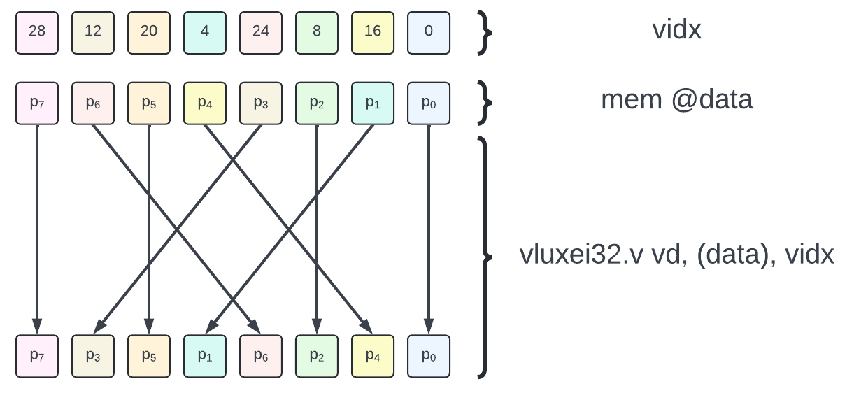
Note: RVV 1.0 offers both unordered (vlux*) and ordered (vlox*) vector indexed loads. Since we are accessing data (and not MMIO) there is no need to enforce specific ordering constraint on the gather accesses. Thus we use the unordered variant ( vlux*).

Optimization: Depending on the implementation, indexed loads can be quite slow. Note that a subset of the element indices match between source and destination (e.g. p0, p2, p5 and p7), thus masks could be leveraged with both indexed and unit-stride accesses to reduce the number of elements which must be randomly gathered. The elements that are invariant through the transform permutation are the ones whose index binary encodings are symmetric (and thus invariant by bit reverse). For a n-element transform, there should be 2^ceil(log2(n) / 2) such coefficients.

To use vector indexed loads we must materialize array of indices. One way to do that is to pre-compute the indices and store them in the program binary. This requires a unit-strided vector load to load indices from memory into a vector register group before using that group as the index operand for the vector indexed loads.

Another technique is to materialize the indices directly through arithmetic computations only. It is well-known that for the FFT/NTT algorithm we use, the index value is the n-bit bit mirroring of the coefficient’s index: for example the index of the 7-th element is: brev(7b0000111) = 7b1110000 = 112. Unfortunately, the 7-bit reverse is not part of the operations supported in RVV 1.0. 8-bit bit reverse was introduced in the vector crypto bit manipulation Zvkb (see the “Bit and Byte reversal” paragraph in our second post on the vector crypto extensions). a 7-bit reversal could be implemented by first performing a 1-bit logical left shift followed by an 8-bit reverse.

Butterfly levels using RVV

Once the coefficients have been permuted, the second stage of the NTT can start: building the k-element NTT from two (k/2)-element NTTs by multiplying by the powers of alpha (twiddle factors) and performing the butterfly coefficient combinations. This phase starts with k=2 and ends with k=n, it consists in log2(n) butterfly steps. It is illustrated in the case n=8 by the diagram below.

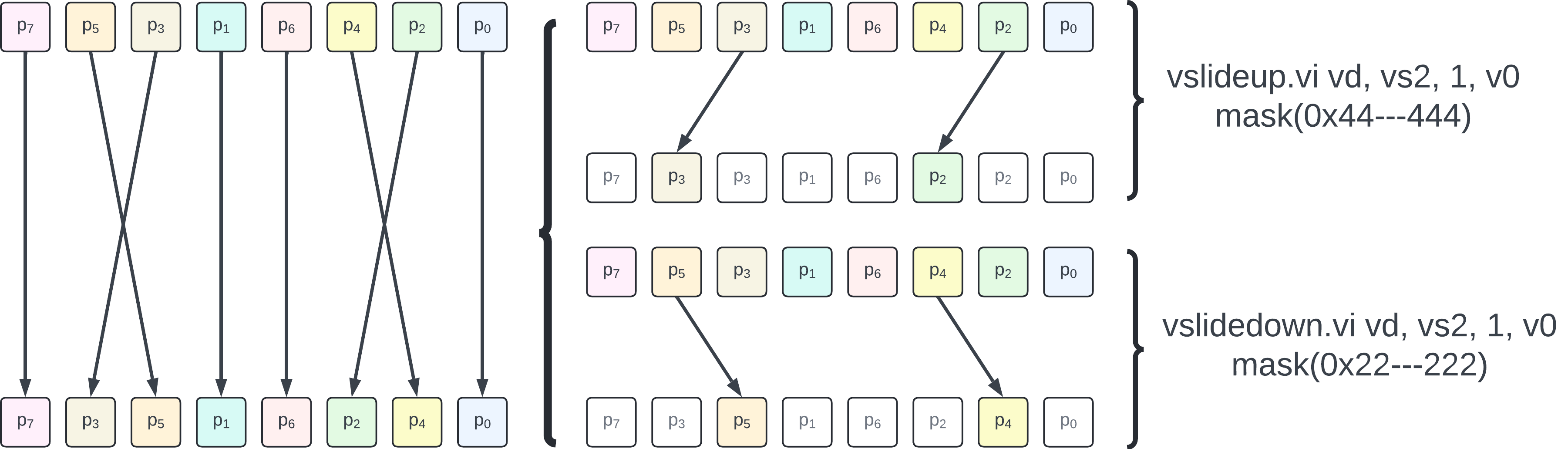
Our RVV implementation splits the butterfly stages into two steps. The first step is applied when n is small; it consists in using a common unit-strided vle instruction to load both even and odd sub-NTT coefficients and then use vslidedown and vslideup instructions with masks to perform the coefficient swap and the butterfly. Operation mappings for the first 3 levels are illustrated below:

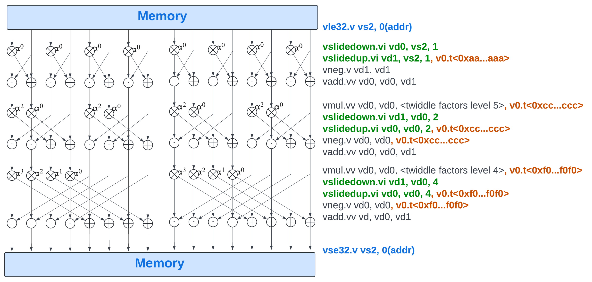
The modulo reductions are not represented on this figure.

Once n is large enough, two separate sets of vle instructions are used: one to load the even sub-NTT coefficient, an other to load the odd sub-NTT coefficient. Once the butterfly pattern has been applied, two separate sets of unit-strided vse instructions are used to store back the results.

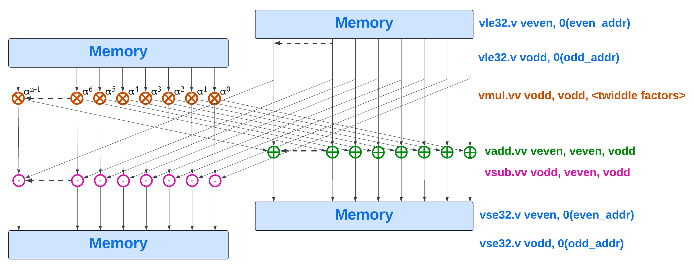
The modulo reductions are not represented on this figure.

Note: depending on the target micro-architecture, it may be faster to used combined multiply-accumulate / multiply-subtract instructions rather than shared a split off vmul.vv. This could have a latency benefit but could draw more power overall if the multiplications by the twiddle factors are computed twice.

NTT multiplication using RVV

This part of NTT is trivial as it maps perfectly to an element-wise multiplication.

Inverse fast NTT

Computing the inverse NTT is simply computing the NTT but using the reciprocal of the root of unit, rather than the root of unity itself, and finally dividing the resulting coefficients by the polynomial degree.

Thus we re-use all the techniques previously described and simply swap the root of unity for its reciprocal (updating the pre-computed tables when required). We append a multiplication by the pre-computed reciprocal of the degree n in Zq.

Note: the division of the result by the polynomial degree can be performed before the inverse transform and fused with the element-wise multiplication in the NTT domain.

Benchmark(eting)

We have implemented a few versions of polynomial multiplication:

• baseline polynomial multiplication: pure scalar C implementation of the quadtric (2-level loops) dummy algorithm.

• fast ntt-based multiplication: pure scalar C implementation of the Number Theoretic Transform. The recursive odd/even split is implemented with a sub-optimal method mixing recursive evaluation of the permuted coefficient index and polynomial splitting (there are certainly some room for improvement here).

• RVV-based ntt-based multiplication: NTT multiplication with minimal use of RVV, only the element-wise multiplication and the scaling by the inverse of the degree are performed using RVV; all the other operations are using the “fast ntt-based multiplication” scalar variant.

• RVV-based ntt-based multiplication recursive: straightforward implementation of NTT based fully based on RVV to implement the “fast ntt-based multiplication” variant.

• RVV-based ntt-based multiplication indexed-load: this variant implements the odd/even split in a single-pass using vector indexed loads and pre-computed destination indices.

• RVV-based ntt-based multiplication strided-load: this variant relies of two sets of vector strided loads to perform the odd/even split.

• RVV-based ntt-based multiplication vcompress: this variant uses a mix of unit-strided vector loads and in-register vcompress.vm instructions to perform the odd/even split.

• RVV-based ntt-based multiplication (fastest variant): this is the (current) fastest of our implementation, it selects all the best techniques from other variants and fuses some of the stages (to avoid storing intermediary data back to memory if multiple steps can be handled in vector registers). This implementation requires LMUL >= 2 for our VLEN-128 as it unrolled some of the butterfly levels which require 8 elements to fit in a vector register group.

The source code for the RVV variants are available in our rvv-examples repository: poly_mult_rvv.c; the scalar variants are available in ntt_scalar.c; and the benchmark wrapper in bench_poly_mult.c.

Note: we also implemented and benchmarked a slow ntt-based multiplication variant: pure scalar C implementation of the number theoretic transform using 2 levels of quadratic loops to compute each coefficients (none of the fast NTT techniques are used). Its performance was abysmal, around 40’000’000 cycles per polynomial multiplication so we excluded it from the results to keep the other variants visible on the vertical axis.

We are comparing the performance of our implementations on real RISC-V hardware, the CanMV K230 v1.1 SBC (Single Board Computer).

make EXTRA_CFLAGS="-I /usr/include/ -O3 -fPIC -DVERBOSE -DNUM_TESTS=10 -DCOUNT_CYCLE" BUILD_DIR=build RISCVCC=clang build/bench_poly_mult

The compiler version is:

clang version 18.1.3
Target: riscv64-unknown-linux-gnu

We have put together a set of C macros (source code) which allow us to modify the LMUL used at compile time without requiring any change in the source code. This opens up the possibility of benchmarking LMUL values.

The benchmark results are plotted below (lower is better):

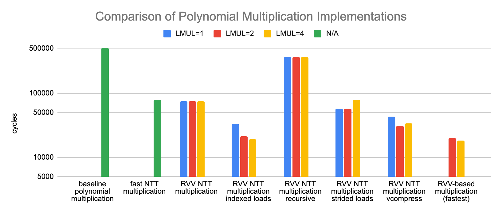
The baseline, dummy, scalar implementations takes more than 500’000 cycles to perform the multiplication of two degree-127 polynomials. This can be taken down to a little under 80’000 cycles with a fast NTT scalar implementation. RVV-based implementations can get this down even further. It seems that using indexed loads is best for the first NTT stage (the permutation) compared to using recursive odd-even splits with either strided vector loads or unit-strided loads and vcompress. For the second stage, the vector remainder instruction seems to be rather slow on our target and using a vectorized Barrett’s reduction method seems to provide better results.

The fastest implementation we tried is about 4 times faster than the fastest scalar implementation we have tried (although I suspect this ratio could be lowered by working on the scalar implementation). The fastest RVV implementation is below 20’000 cycles with an intrinsic only implementation (no assembly).

Sub-benchmark: Barrett vs vrem

We have performed a small experiment: using vrem.vx rather than Barrett’s reduction to perform the modulo operation after multiplying coefficients together or multiplying coefficients with twiddle factors (or with the inverse of the degree).

The results are reported below (lower is better):

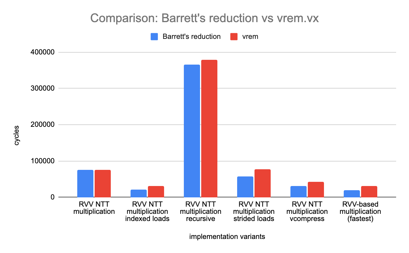
On the K230, the result is a landslide: our implementation of Barrett’s reduction is always better than using vrem.vx directly. The speed-up varies between a few percent for “RVV NTT multiplication” to more than 50% for our fastest variant (31’000 cycles on average when using vrem.vx versus less than 20’000 using Barrett’s reduction).

Conclusion

The Number Theoretic Transform is a very fun and powerful algorithm, it brings down the real life complexity of polynomial multiplication substantially and is a key feature in some of the most notable PQC algorithms. Mapping it over RISC-V Vector shows that some speed-up can be obtained (Although I am not going to claim none of my implementations are anything near optimal, they could still be optimized quite a lot, but this will be a story for another post). The next step is going to be to push optimization further, certainly by implementing some of the sections directly in assembly, but also exploring other techniques.

References:

• Number Theoretic Transform and Its Applications in Lattice-based Cryptosystems: A Survey, Zhichuang Liang and Yunlei Zhao

• CRYSTALS-Dilithium specification, v3.1 dilithium-specification-round3-20210208.pdf

• CRYSTALS-Kyber specification, v3.01 kyber-specification-round3-20210131.pdf

• Blog post on NTT for Kyber and Dilithium: https://electricdusk.com/ntt.html

• rvv-examples repository directory with polynomial multiplications implementations and benchmarks: https://github.com/nibrunie/rvv-examples/tree/main/src/polynomial_mult