
Implementing Softmax using RISC-V Vector
Quick and dirty method to implement a vectorized non-linear function using RVV

Updated Feb 22nd 2024: a tighter polynomial (many thanks to Eric B. and Hugues for pointing it my mistake on the original approximation interval).
Updated Mar 2nd 2024: fixing a double typo (thank you to Superkoning for pointing it out).
Softmax activation function in a nutshell
Softmax is a non-linear normalization layer used in neural networks. It consists in computing the exponential of each element of a tensor and then dividing the result by the sum of exponential of all the input elements.
Note: as always with neural network “all the elements” may be reduced to a sub-space of the input tensor. For example normalizing a 2D tensor and only summing the exponentials across one dimension. In this post we describe the implementation of softmax on a 1D array.
Let us assume aᵢ is a n-element input vector and let us write the equation for Sᵢ, the softmax function for the i-th element:
Numerical Stability Consideration
The exponential function grows rapidly (some would say exponentially !) with the input values and for standard floating-point formats it can overflow rapidly: in binary32 / single precision exponential overflows for an input slightly greater then 88.0 and in binary16 / half precision it overflows around 10.4.
If we try to sum raw exponential results we may end up overflowing to +infinity pretty easily.
One well know fact about softmax is the you can divide both numerator and denominator by:
to get
And now, every exponential is computed on a negative or zero value, making it much well numerically behaved.
We are first going to implement the naive formula using RISC-V Vector (RVV). Then we will refine our implementation to implement the more stable second formula. The second formula should have a performance cost (since it adds evaluation of the maximum) that we will evaluate.
The next section, “Exponential Approximation“, presents a method to build an approximation scheme for the exponential (a scheme that is easy to vectorize). The actual vectorization is presented in the section “Building a Vector Softmax“.
Exponential Approximation
To compute softmax we need a way to compute the exponential function. There is quite an extensive literature on the approximation of elementary function. If you are looking for an in-depth introduction I would recommend Jean-Michel Muller’s Elementary Function: Algorithms and Implementations. Here we will use a standard decomposition:
Argument reduction: convert the function input x to another argument t in a smaller range such that exp(x) becomes g(f(t)) with functions g and f selected properly
Polynomial approximation: approximate f(t) using a polynomial. Polynomials are easy to implement with FMA and are often a good fit for FPUs and vector FPUs.
Reconstruction: reconstruct exp(x) using the function g and the approximation of f(t)
Exponential Argument Reduction
The exponential argument reduction we are going to use on the fact that computing 2^i, with i an integer, is trivial in floating-point arithmetic. We split the input x into an integer multiple of ln(2) (easy to exponentiate) and a much smaller reduced argument r as follows:
Note that this is a theoretical formula that we will approximate (with errors) using floating-point arithmetic.
we will approximate ln(2) by the constant ln2 and 1/ln(2) by the constant iln2.
k = nearbyint(x * inl2) // rounding to the closest integer
r = x - k * ln2         // computing the reduced argument
The expression for r should actually be implemented using a Fused Multiply-Add (FMA) a floating-point operation able to compute x - k * ln2 with only a final rounding (and no intermediary rounding of the product). Using an FMA greatly improves the accuracy of r.
From the argument reduction, it will be easy to reconstruct exp(x).
Since k is an integer 2 ^ k simply corresponds to injecting an exponent in a floating-point number (discarding overflows and underflows).
Exponential Approximation on [-ln(2)/2, ln(2)/2]
Now we need to approximate exp(r). x was on [-inf, 88], and r in on [-ln(2)/2, ln(2)/2].
Many different methods exist to evaluate such a polynomial approximation and you can do much better than a default Taylor approximation. The metrics we are trying to optimize for are many:
small degree
low approximation error
We also want the polynomial to have a “nice” numerical behavior, since eventually we will implement it using floating-point arithmetic (and not real number arithmetic).
A very good tool to compute accurate approximation polynomial is the Sollya library, which also provides highly optimized and accurate methods to compute approximation error.
We are going to use sollya through pythonsollya, a python wrapper.
Let’s first load sollya into a python interpreter and configure it:
>>> import sollya
>>> sollya.settings.display = sollya.hexadecimal
We then define a few variables useful for our problem:
>>> ln2ov2 = sollya.round(sollya.log(2)/2, sollya.binary32, sollya.RN)
>>> approxInterval = sollya.Interval(-ln2ov2, ln2ov2)
>>> approxFunc = sollya.exp(sollya.x)
>>> iln2 = sollya.round(1/sollya.log(2), sollya.binary32, sollya.RN)
>>> ln2 = sollya.round(sollya.log(2), sollya.binary32, sollya.RN)
>>> iln2, ln2
(0x1.715476p0, 0x1.62e43p-1)
We can then use Sollya’s implementation of the fpminimax algorithm to compute a degree 6 polynomial approximation to exp(x) with single precision coefficients:
>>> degree = 6
>>> poly = sollya.fpminimax(approxFunc,
                            degree,
                            [1] + [sollya.binary32] * degree,
                            approxInterval)
0x1p0 + _x_ * (0x1p0 + _x_ * (0x1.fffff8p-2 + _x_ * (0x1.55548ep-3 + _x_ * (0x1.555b98p-5 + _x_ * (0x1.123bccp-7 + _x_ * 0x1.6850e4p-10)))))
Note: the 3rd argument to sollya.fpminimax is the list of coefficient formats. We force the force coefficient to a single bit of precision which has the indirect effect of forcing it to 1.0 (fpminimax also accepts direct coefficient values).
Sollya can also be used to compute an interval around the approximation error:
>>> sollya.supnorm(poly, approxFunc, approxInterval, sollya.relative, 2**-53)
[0x1.fbad01f097c2f3644cp-29;0x1.fbad01f097c302c2c8cf089826de494dp-29]
The relative approximation error of our polynomial approximation is around 2^-26
Scalar implementation of exponential
Let us first start with a simple scalar implementation. Beware that this implementation is quick and dirty: it does not return an accurate result on the full range of floating-point numbers:
float quick_dirty_expf(float x) {
    const float ln2 = 0x1.62e43p-1;
    const float iln2 = 0x1.715476p0f;

    // argument reduction
    const int k = nearbyintf(x * iln2);
    const float r = fmaf(- k, ln2, x);

    // polynomial approximation exp(r)
    const float poly_coeffs[] = {
        0x1p0,
        0x1.fffff8p-2,
        0x1.55548ep-3,
        0x1.555b98p-5,
        0x1.123bccp-7,
        0x1.6850e4p-10,
    };

    // Horner evaluation scheme for the degree 6 polynomial
    // 1 + x * (c_1 + x * (c_2 + ...)
    float poly_r = poly_coeffs[5];
    int i = 0;
    for (i = 4; i >= 0; i--) {
        // poly_r = poly_r * r + poly_coeffs[i];
        poly_r = fmaf(poly_r, r, poly_coeffs[i]);
    }
    // poly_r = 1 + r * poly_r;
    poly_r = fmaf(r, poly_r, 1.f);


    // quick and dirty (does not manage overflow/underflow/
    // special values) way to compute 2^k by injecting the
    // biased exponent in the proper place for IEEE-754
    // binary32 encoding.
    uint32_t exp2_k_u = (127 + k) << 23;

    // casting from uint32_t to float (reinterpreting bits)
    // using a union here is a undefined behavior (accessing
    // two different fields) so I think the proper way to do it
    // is through a memcpy which will be optimized away by any
    // modern compiler
    float exp2_k;
    memcpy(&exp2_k, &exp2_k_u, sizeof(float));

    // result reconstruction
    float exp_x = poly_r * exp2_k;

    return exp_x;
}
There are a few things to note.
const int k = nearbyintf(x * iln2);First of all in the argument reduction, we need to convert a floating-point value to the closest integer and have the result in both floating-point and integer forms. The function nearbyintf from the standard math library provide the floating-point result. Its result is converted to an integer to be used in the reconstruction. Given the possible range of values here, the conversion is always exact.
const float r = fmaf(- k, ln2, x);We use the function fmaf (also from the standard library) to enforce the use of an FMA operation to evaluate the reduced argument.
For the evaluation of the polynomial approximation on the reduced argument we use a Horner scheme: coeff_0 + x( coeff_1 + x * (coeff_2 + x * …). We won’t go into the numerical quality of this evaluation scheme (it is often more accurate for the type of polynomial with decreasing coefficients value we use here). An important thing to know is that it minimizes the number of operations compared to some schemes which expose more parallelism (e.g. Estrin’s). This means that it may exhibit a longer latency but is better suited for throughput oriented implementation (generally a good fit for vector).
Concerning the reconstruction, we have used a dirty trick to compute 2^k which is not really recommended except if one can determine that the range of k is compatible with it: if k + 127 = 255 we get infinity and if k + 127 > 255 then the result is completely invalid (e.g. negative which could be partially solved by masking).
Measuring our implementation accuracy
We have compared our quick and dirty implementation of exponential to the standard double precision exp function (used as golden). We report below the results between -10 and 5:
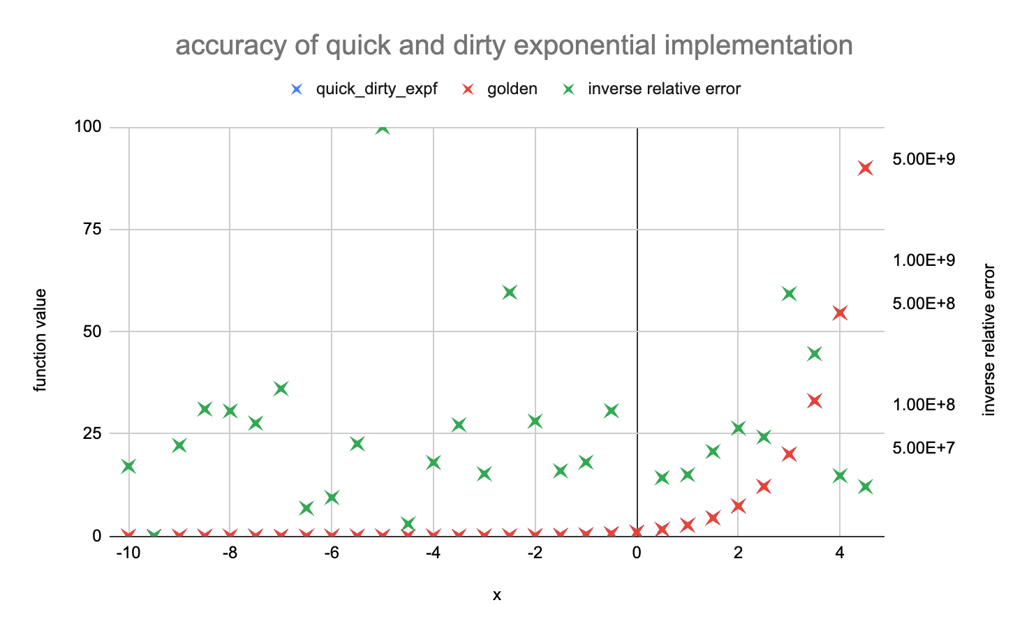
The left axis corresponds to the function values. quick_dirty_expf (blue cross) and golden (red cross) can not be distinguished and seem to overlap on the full range. We have also plot in green the inverse of the relative error of quick_dirty_expf versus the golden reference implementation.
Between -10 and 5, the relative error between our implementation and the double precision exp function is smaller than 1e-7 (some outliers are missing from the chart above) and is on average about 2.5e-8: we get more than 23 bits of accuracy.
Note: our quick and dirty approximation is only accurate between -86 and 88, outside this range it diverges a lot (really a lot) from the expected value. This is the price for a dirty approximation.
Building a Vector Softmax
Let us now use our hand-made approximation of exponential to implement the softmax function:
Note: Our first version of vector softmax does not subtract the maximum of the input array before evaluating the exponential function.
Building a Vector exponential (with sum)
To build a vector softmax we are going to buikd a vectorized implementation of exponential which also returns the sum of its results.
float quick_dirty_vector_expf(float* dst, float* src, size_t n);The complete function definition can be found in the repository associated with this post at rvv-examples/src/softmax/softmax_rvv.c#L88.
Let us start with definitions of some constants and an accumulation variable for the sum of exponentials (we use a vector accumulator):
const float ln2 = 0x1.62e43p-1;
const float iln2 = 0x1.715476p0f;

const size_t vlmax = __riscv_vsetvlmax_e32m1();
const vfloat32m1_t vln2 = __riscv_vfmv_v_f_f32m1(ln2, vlmax);
const vfloat32m1_t viln2 = __riscv_vfmv_v_f_f32m1(iln2, vlmax);

// element-wise reduction accumulator
vfloat32m1_t vsum = __riscv_vfmv_v_f_f32m1(0.f, vlmax);

// (const) attributes removed to fit in substack default code block
vfloat32m1_t poly_c_0 = __riscv_vfmv_v_f_f32m1(0x1.p0, vlmax);
vfloat32m1_t poly_c_1 = __riscv_vfmv_v_f_f32m1(0x1p0, vlmax);
vfloat32m1_t poly_c_2 = __riscv_vfmv_v_f_f32m1(0x1.fffff8p-2, vlmax);
vfloat32m1_t poly_c_3 = __riscv_vfmv_v_f_f32m1(0x1.55548ep-3, vlmax);
vfloat32m1_t poly_c_4 = __riscv_vfmv_v_f_f32m1(0x1.555b98p-5, vlmax);
vfloat32m1_t poly_c_5 = __riscv_vfmv_v_f_f32m1(0x1.123bccp-7, vlmax);
vfloat32m1_t poly_c_6 = __riscv_vfmv_v_f_f32m1(0x1.6850e4p-10, vlmax);
fesetround(FE_TONEAREST);
The variable vsum is going to be used to accumulate the exponential results computed in the main loop through an element-wise addition before eventually reducing it to a single sum result in the loop epilog.
Note: splitting the reduction into an element-wise operation in the loop body and a final reduction outside of the loop should be faster on real hardware than reducing it to a single element in each iteration of the loop.
The final line of the previous snippet makes sure the floating-point rounding mode is set to round-to-nearest (tie-case to even) as we need to enforce this rounding mode in particular when computing the closest integer to x * iln2.
Let us continue with the main loop which iterates over all the inputs, vl elements at a time:
size_t avl = n;
while (avl > 0) {
    size_t vl = __riscv_vsetvl_e32m1(avl);
    vfloat32m1_t vx = __riscv_vle32_v_f32m1(src, vl);
Argument reduction:
    // argument reduction: x * 1 / log(2)
    vfloat32m1_t vxiln2 = __riscv_vfmul(vx, iln2, vl);
    // k = integer(x * iln2); require round to nearest mode
    vint32m1_t       vk = __riscv_vfcvt_x_f_v_i32m1(vxiln2, vl);
    vfloat32m1_t    vfk = __riscv_vfcvt_f_x_v_f32m1(vk, vl);
    // using vfnmsac.vf to evaluate r = x - k * log(2)
    vfloat32m1_t     vr = __riscv_vfnmsac(vx, ln2, vfk, vl);
RVV does not provide a direct instruction to convert a floating-point value to the nearest integer (with the result in floating-point format, such a the scalar fround instruction added in the Zfa extension). We have to rely on a conversion to integer and a conversion back to floating-point. The first conversion performs the rounding and the second conversion is exact (given the input range): it simply change the value format.
With the reduced argument vr we can compute the polynomial approximation:
    // polynomial approximation exp(r)
    vfloat32m1_t poly_vr = poly_coeffs_6;
    poly_vr = __riscv_vfmadd(poly_vr, vr, poly_c_5, vl);
    poly_vr = __riscv_vfmadd(poly_vr, vr, poly_c_4, vl);
    poly_vr = __riscv_vfmadd(poly_vr, vr, poly_c_3, vl);
    poly_vr = __riscv_vfmadd(poly_vr, vr, poly_c_2, vl);
    poly_vr = __riscv_vfmadd(poly_vr, vr, poly_c_1, vl);
    poly_vr = __riscv_vfmadd(poly_vr, vr, poly_c_0, vl);
We finalize the exponential evaluation with the reconstruction:
    // reconstruction
    const int exp_bias = 127;
    // biased_exp = vk + 127
    vint32m1_t vbiased_exp = __riscv_vadd(vk, exp_bias, vl);
    // exp2_vk = 2^vk
    vint32m1_t vexp2_vk    = __riscv_vsll(vbiased_exp, 23, vl);
    // casting 2^k into a vector of floating-point elements
    vfloat32m1_t vfexp2_vk;
    vfexp2_vk = __riscv_vreinterpret_v_i32m1_f32m1(vexp2_vk);

    vfloat32m1_t vexp_vx  = __riscv_vfmul(poly_vr, vfexp2_vk, vl);
As presented in our post “RISC-V Vector Programming in C with intrinsics”, the reinterpret function does not generate an actual instruction: it is simplified away by the compiler and is used to redefine how the same vector data should be interpreted.

We accumulate the results into the temporary sum vector accumulator:
vsum = __riscv_vfadd_vv_f32m1_tu(vsum, vsum, vexp_vx, vl); For the element-wise addition used for the temporary reduction, RVV tail-undisturbed mode is mandatory. It ensures that, in the case vl < VLMAX, unaffected sum terms in vsum are not modified by the instruction.
We finish the loop body by storing the new results and updating the application vector length and the source and destination pointers:
    __riscv_vse32(dst, vexp_vx, vl);
    avl -= vl;
    src += vl;
    dst += vl;
In the loop epilog, we reduce the temporary accumulator to a single result using RVV’s reduction operation, vfredusum:
vfloat32m1_t vredsum = __riscv_vfmv_v_f_f32m1(0.f, vlmax);
vredsum = __riscv_vfredusum_vs_f32m1_f32m1(vsum, vredsum, vlmax);

float sum = __riscv_vfmv_f_s_f32m1_f32(vredsum);
RVV offers two variants of floating-point reduction sum: vfredusum and vfredosum. They differ by the evaluation ordering constraint. vfredusum is unordered and does not mandate any operation ordering, leaving more freedom to hardware implementations. vfredosum is ordered and mandates that the active elements be accumulated in order (with a rounding after each 2-operand addition) starting with the accumulator element (from vs1).
We have selected the unordered variant (favoring performance over predictable accuracy).
Assembling a RVV softmax implementation
The vectorized exponential with sum was the most complex block. With it in hand, it is pretty easy to build together a softmax implemenation (the full source code can be found at rvv-examples/src/softmax/softmax_rvv.c#L207):
void softmax_rvv_fp32(float* dst, float* src, size_t n)
{
    // computing element-wise exponentials and their seum
    float sum = quick_dirty_vector_expf(dst, src, n);

    // computing the reciprocal of the sum of exponentials,
    // once and for all
    float inv_sum = 1.f / sum;

    // normalizing each element
    size_t avl = n;
    while (avl > 0) {
        size_t vl = __riscv_vsetvl_e32m1(avl);
        vfloat32m1_t row = __riscv_vle32_v_f32m1(dst, vl);
        row = __riscv_vfmul_vf_f32m1(row, inv_sum, vl);
        __riscv_vse32(dst, row, vl);
        avl -= vl;
        dst += vl;
    }
}
Improving RVV softmax stability
Now that we have a baseline full-RVV implementation, we can address the implementation of the second formula for softmax:
The complete code can be found at rvv-examples/src/softmax/softmax_rvv.c#L239.
void softmax_stable_rvv_fp32(float* dst, float* src, size_t n)
{
    // initializing temporary maximum vector
    // vlmax initialization is required in case the first vsetvl does
    // not return VLMAX while avl > vl: in this case we need to
    // avoid some uninitialized values in vmax
    const size_t vlmax = __riscv_vsetvlmax_e32m1();
    vfloat32m1_t vmax = __riscv_vfmv_v_f_f32m1(-INFINITY, vlmax);

    size_t avl = n;
    size_t vl = __riscv_vsetvl_e32m1(avl);
    vmax = __riscv_vle32_v_f32m1_tu(vmax, src, vl);
    avl -= vl;
    src += vl;

    while (avl > 0) {
        size_t vl = __riscv_vsetvl_e32m1(avl);
        vfloat32m1_t vx = __riscv_vle32_v_f32m1(src, vl);
        vmax = __riscv_vfmax(vx, vmax, vl);
        avl -= vl;
        src += vl;
    }
    src -= n; // reseting source pointer

    // final maximum reduction
    vfloat32m1_t vredmax = __riscv_vfmv_v_f_f32m1(0.f, vlmax);
    vredmax = __riscv_vfredmax(vmax, vredmax, vlmax);
    float max_x = __riscv_vfmv_f_s_f32m1_f32(vredmax);

    // subtracting max_x from each source element
    avl = n;
    while (avl > 0) {
        size_t vl = __riscv_vsetvl_e32m1(avl);
        vfloat32m1_t row = __riscv_vle32_v_f32m1(src, vl);
        row = __riscv_vfsub(row, max_x, vl);
        __riscv_vse32(src, row, vl);
        avl -= vl;
        src += vl;
    }
    src -= n; // reseting source pointer
After this, we can simply call our baseline implementation on the normalized array:
    softmax_rvv_fp32(dst, src, n);
}
Benchmark(et)ing
We have put together a benchmark to evaluate some performance metric and the accuracy of our various implementations (and some variants not described here). The code for the benchmark is available at rvv-examples/src/softmax/bench_softmax.c.
We have used the riscv-isa-sim (spike) simulator to count the number of retired instructions in our implementations. Although this metric can be very inaccurate for performance improvements, I think it still represents an interesting point of comparison. In particular in the case of a arithmetic heavy function such as softmax. None of the implementations make an heavy use of memory and all are pretty arithmetic intensive and so should run at close to peak throughput (assuming long enough vl and discarding some memory hierarchy effects when accessing arrays linearly).
We have benchmarked our softmax implementations on various sizes of input array ranging from 4 elements to 512 elements. For each array size we have measured performance and accuracy on 100 random arrays of elements between -2 and 2.
The results are reported below, in absolute numbers (lower is better) and in element per cycle (higher is better) which we use as a metric for throughput.
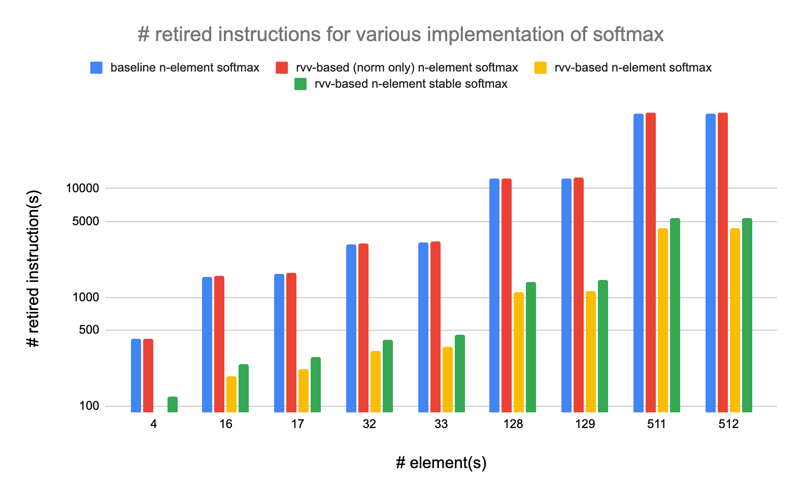
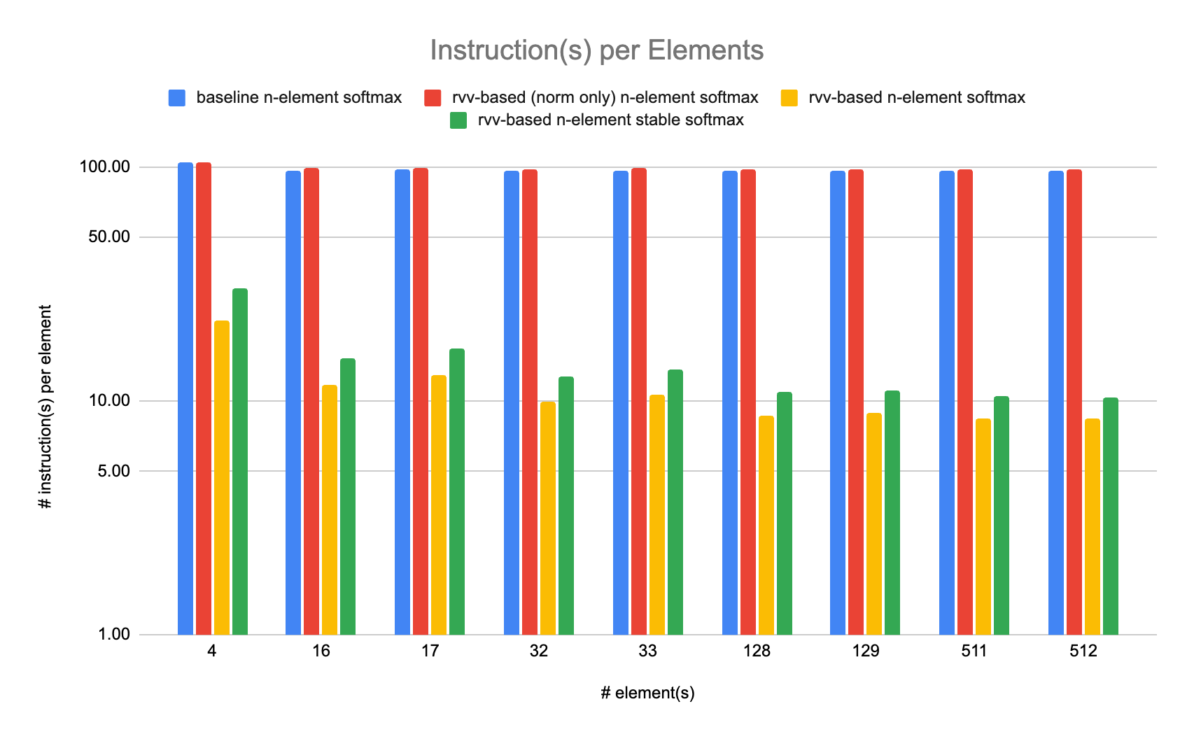
We can see that the RVV-based implementations are much faster that our naive implementations based on expf. On large array sizes, the fastest rvv-based softmax reaches around 8.5 retired instructions per element and the more numerically stable rvv-based softmax reaches around 10.5 retired instructions per element: numerical stability cost about 2 extra retired instructions per element (about 23.5% increase).
The accuracy of the implementations under test is evaluated against a golden model consisting of the baseline implementation (not using RVV explicitly) in double precision. For a given number of elements, the variants are executed on the same inputs (100 random arrays).

In our experiments, the stable rvv-based softmax is often less accurate than the “unstable” version. Overall the RVV-based implementations seem numerically sound compared to the baseline. In particular the errors of RVV-based implementation become smaller than the baseline for larger arrays. After some investigation, it seems that this is related to the parallel accumulation of exponential results: rvv-based (vanilla and stable) implementations use multiple accumulators while the baseline and norm-only use a single accumulator; the multi-element accumulator improve the accuracy of the sum and provide a result closer to the golden value.
Conclusion
RVV is well suited to implement vector elementary functions and even more advanced functions such as softmax. We have shown that it was possible to implement an accurate softmax with competitive performance in front of a naive baseline implementation.
Our implementation could benefit from a few extra instructions (e.g. vfround) although the performance effect should be limited. It can be easily tuned to lower precision by modifying the degree of the polynomial approximation which should provide various performance/accuracy compromises.
We have made use of some reduction operations while mostly relying on element-wise operations for the bulk of or reductions. In such case, it is important to properly initialize temporary accumulators using VLMAX and proper identity values. Doing so ensures that the computation is correct whatever the actual vector lengths.
References:
Source code of implementations and benchmarks: rvv-examples/src/softmax
Reference book on computer arithmetic for elementary functions: Jean-Michel Muller’s Elementary Function: Algorithms and Implementations
Building a Numerically Stable Softmax, Brian Lester